Recently, there has been considerable interest in studying biophysical neural networks using methods from statistical physics like mean field theory and random matrix theory. In Sompolinsky, Crisanti, & Sommers, 1988, a toy model of a neural network composed of an infinite number of neurons was modeled by coupled first-order differential equations of the extracellular potentials with respect to time. They found that when the synaptic weights and input gain of each neuron are drawn from a (uncorrelated) normal distribution that there exists a threshold value of the gain where the network transitions from steady-state (the extracellular potential saturates like an overdamped oscillator) to chaotic (sustained oscillations that are sensitive to the initial conditions). Since Sompolinsky, et al, several extensions have been made to the network model to study the properties of increasingly more realistic (and more difficult) scenarios. For instance, the work of Aljadeff, Stern, & Sharpee introduced different distributions for the synaptic weights based on neuron type instead of a universal normal distribution. Others have made changes to the differential equations describing the individual neurons by introducing a more realistic spiking model like Rubin, Abbott, & Sompolinsky.

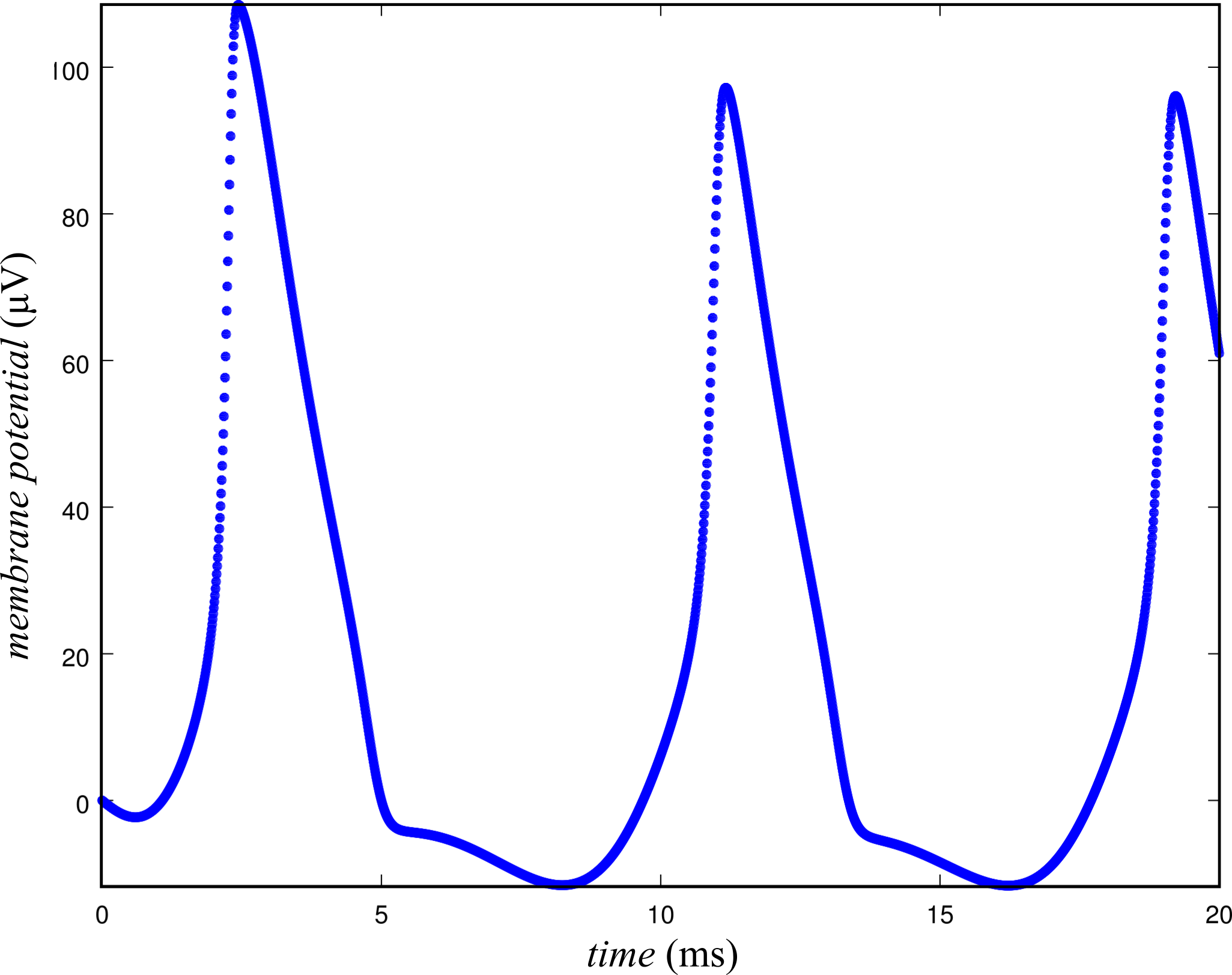
In the following analysis, I decided to take a look at a more complicated spiking neuron model than those studied in the prior papers: the classic Hodgkin-Huxley model for the potential difference across the membrane of an excitable tissue. In my case, I use the Hodgkin-Huxley model to approximate the membrane potential of a neuron. An empirical approach is used to explore whether Hodgkin-Huxley based neural network has a demonstrable phase transition from steady state to chaos as a function of the gain consistent with the predictions Sompolinsky, et al made on the simpler toy models.

The Hodgkin-Huxley model is a nonlinear differential equation of the form

where \( V \) is the membrane potential as a function of time, \( C \) is the membrane capacitance (per unit area), \( g_\mathrm{K} \) and \( g_\mathrm{Na} \) are the conductances (per unit area) of the potassium and sodium ion channels, respectively, \( g_\mathrm{l} \) is the conductance (per unit area) of the "leakage" current, \( V_\mathrm{K} \), \( V_\mathrm{Na} \), and \( V_\mathrm{l} \) are the reversal potentials of the ion channels and leakage current, and finally \( I^\mathrm{(ext)} \) is an external current that corresponds to the in and out-flow of current from the extracellular medium due to external sources and sinks. Note that this equation is equal to zero due to charge conservation.

Now, if one were to assume that, in the absence of external current, this is simply a first-order differential equation that can be solved analytically, he/she would be wrong. This is because the ion channel conductances themselves are membrane voltage-dependent (excluding the leakage conductance, which is typically held constant) which makes physiological sense since the ion channels are inhibited as a neuron depolarizes. The conductances are often modeled by the equations

with the ion channel activations \( n \), \( m \), and \( h \) being governed by the first-order differential equations

For definitions of the nonlinear equations for the rate coefficients, \( \alpha_j \) and \( \beta_j \), see this Wikipedia article. These rate equations were used in this work along with Hodgkin & Huxleys' settings for the constants (see function init_lit() in hhnet.c for the values). These same settings are used for all neurons in the network.

Each of the \( N \) neurons in the network are described by their own Hodgkin-Huxley model. The neurons are coupled by the their synaptic connections through \( I \) leading to a \( N \) coupled differential equations that need to be solved. In this case, the external current received by the \( i \)th neuron from the other neurons in the network is modeled by a logistic function

where the bracketed terms in the denominator prevent divergence of the membrane potential (which is reasonable since there is a limited number of ions in the immediate extracellular media). The \( N \times N \) matrix \( \mathbf{J} \) is a random matrix of synaptic weights where \( J_{i,j} \) is the synaptic weight of signal from the \( j \)th neuron to the \( i \)th neuron. The elements \( J_{i,j} \) are drawn from a normal distribution with mean zero and variance \( \sigma^2 \) where \( \sigma \geq 0 \) will be called the "gain". The diagonal elements of \( \mathbf{J} \) are set to zero to prevent self-stimulation self-stimulation. The \( N \times N \) matrix \( \mathbf{T} \) is matrix of transmission time delays where the element \( T_{i,j} \) is the time it takes for signal to travel along the axon of the \( j \)th neuron to the dendrites of the \( i \)th neuron. The elements \( T_{i,j} \) are drawn randomly from a uniform distribution on the domain [0 ms, 500 ms]. Note that \( T_{i,j} \) must be greater than or equal to zero due to causality. The remaining parameters in \( I_i^\mathrm{(trans)} \)(t) are: \( a_\mathrm{in} = 50.0 \), \( a_\mathrm{out} = 75.0 \), \( b_\mathrm{in} = 1.0 \), and \( b_\mathrm{out} = 1.0 \).

Instead of beginning the simulation of the network from a random network state, the network is initialized to a silent state (i.e. \(V_i(t \leq 0) = 0\) for all \(i \in \left\{1, \cdots, N \right\}\)) and a brief episode of external stimulation is used to give the network a "jolt". Two forms of stimulation are provided by default in hhnet.c. The first is a sudden impulse or "hit" of \( 2,000 \, \mathrm{\mu V}\) constant current that lasts only one time step (function hit_stim()) and the second is a sum of two sine waves with different (user-defined) amplitudes, wavelengths, and phases. These two stimulus currents can be expressed by the following two equations:

where \( \Theta(\cdot) \) is the Heaviside step function, \(t_0 \) is the stimulus onset time, and \( \Delta t \) is the impulse duration. The parameters defining the sinusoidal stimulus have their typical definitions in terms of amplitude, wavelength, and phase. The total input current incident on a given neuron is the sum of the transmission currents and external stimuli, \( I_i(t) = I_i^\mathrm{(trans)}(t) + I_i^{(stim)}(t) \)

Clearly, this is a complicated set of nonlinear, coupled differential equations that is not likely to have analytic solution. Therefore, I used a numerical integration technique to approximate the voltage drop across the membrane of each neuron. While Runge-Kutta was the method originally used by Hodgkin-Huxley and many since, I chose to use a simpler method called leapfrog integration for the sake of expediency. Leapfrog integration works as follows using a constant time step, \( \mathrm{d}t^* \):

1. Compute \( I_i^\mathrm{(ext)}(t^*) \text{ for all } i \in \{1, \cdots, N \}\) at time \( t = t^* \).
2. Integrate the channel activation functions a half-step forward in time via \( x_i(t^* + \frac{\mathrm{d}t^*}{2}) = x_i(t^*) + \frac{\mathrm{d}t^*}{2} \frac{\mathrm{d}x_i}{dt} \big|_{t^*} \) for all \( x_i \in \{m, n, h\} \) and all \( i \in \{1, \cdots, N \} \).
3. Integrate the membrane potentials a full-step forward in time using the updated half-step channel activations from step 2 and the external currents from step 1 in \( V_i(t^* + \mathrm{d}t^*) = V_i(t^*) + \mathrm{d}t^* \frac{\mathrm{d}V_i}{\mathrm{d}t} \big|_{t^*} \) for all \( i \in \{ 1, \cdots, N \} \).
4. Integrate the channel activation functions one more half-step forward in time via \( x_i(t^* + \mathrm{d}t^*) = x_i(t^* + \frac{\mathrm{d}t^*}{2}) + \frac{\mathrm{d}t^*}{2} \frac{\mathrm{d}x_i}{\mathrm{d}t}\big|_{t^* + \frac{\mathrm{d}t^*}{2}} \) using the results of steps 2 and 3 over all \( x_i \) and \( i \) as defined in step 2.
5. Update \( t^* \leftarrow t^* + \mathrm{d}t^* \) and repeat all of the above steps.

Figure 1: three spikes were simulated using leapfrog integration for a single neuron stimulated by an external sinusoidal current. Note that \( V \) is negated from the convention in used the equations where spikes are negative.

To show whether a transition between domains of steady-state and chaotic network dynamics occur as a function of the gain, a network of \( N = 100 \) neurons was simulated with different values of the gain, \( \sigma \), tried on the range \( \left[0, 1000 \right] \mathrm{\mu V} \). To ensure that the network activity was not the result of external stimulation, a sinusoidal stimulus was only applied for the first 10 ms of the simulation. Furthermore, the external stimulus was only applied to one neuron to demonstrate that the spiking activity that was observed for other neurons in the network was a result of transmission between neurons. To illustrate more clearly what is meant by steady-state and chaos, simulations were performed with low and high gain and plotted in Figures 2 & 3, respectively.

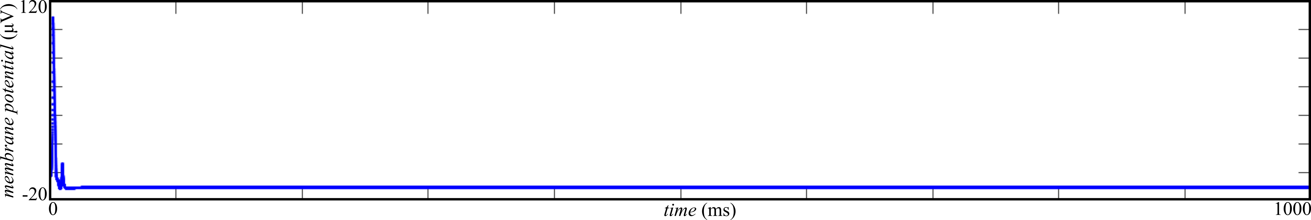Figure 2: steady-state activity is observed for \( \sigma = 10 \mathrm{\mu V} \). Following 10 ms of external stimulation, all neurons in the network decay immediately to baseline activity.

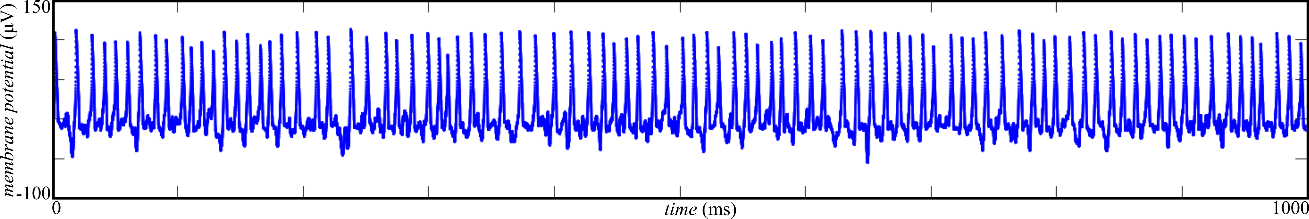Figure 3: chaotic activity is observed for \( \sigma = 1000 \mathrm{\mu V} \). After 10 ms of external stimulation, the network exhibits self-sustained spiking at least up to 1000 ms.

At each value for the gain, the simulation was repeated 100 times with newly generated random synaptic weights and time delays. Whether the simulation resulted in steady-state or chaotic network activity for each of these trials was determined automatically. If the membrane potentials above \( 50 \mathrm{\mu V} \) were observed in the last 50 ms of the simulation, the trial was judged to be chaotic (see Figure 3); otherwise, it was called steady-state (see Figure 2). With chaotic activity denoted by 1 and steady-state activity denoted by 0, these Boolean values were averaged across trails for each gain setting. The probability of a chaotic activity given the gain, \( P(\mathrm{chaotic}|\sigma) \), is plotted in Figure 4.

Figure 4: averaged over 100 trials, there is an apparent phase transition between steady-state and chaos as a function of the gain.

These results appear to provide empirical evidence for a phase transition between steady-state and chaotic dynamics of Hodgkin-Huxley neural networks. The transition has a logistic-esque form with a decision boundary around \( 575 \mathrm{\mu V} \). These results are consistent with the predictions made by Sompolinsky, et al and provide further justification for studying simpler models to learn about biophysical neural network dynamics.