Generally speaking, autoencoders can be used to reduce the dimensionality of ordered data by decomposing data into recurring patterns. Autoencoders can be used as a form of either lossy or lossless compression; though it should be noted that lossless compression is unlikely to lead to a dimensionally reduced model when the data is noisy or composed of more patterns than total dimensions (this problem is not unique to autoencoders, however). Convolutional autoencoders do the same thing under the assumption that patterns are translationally invariant. For instance, cars appearing in a series of pictures may exist in many possible locations within (or across the edge of) a photograph; yet the patterns describing a car should be location-independent. Thus, convolutional autoencoders can further compress the encoding of data by assuming the existence of tranlationally invariant patterns.
In this implementation, the autoencoder is modeled as a convolutional feed-foward neural network as shown in Figure 1.

Each of the layers is fully connected along the forward direction of information flow with logistic activation functions. The convolution layer is composed of \( K \) patches of the data (e.g. images, spectrograms, etc.) which are projected onto the set of weights \( \left\{ \mathbf{w}_i | \text{ for all } i \in \{ 1, \cdots, J \} \right\} \) with biases \( \left\{ a_i | \text{ for all } i \in \{ 1, \cdots, J \} \right\} \). The output of the convolution layer passes as input to either the output layer or to the next hidden layer (if one exists). The output of each hidden layers passes to the next sequential layer as input until reaching the output layer. The output layer has a linear activation function with output the same dimensionality as the input data. The quality of the optimized weights is determined by a least squares comparison of the output layer to the input data.
As an example application, spectrograms generated from President John F. Kennedy's inaugural address (the one famous for the line "ask not what your country will do for you, but what you will do for your country...") will be compressed using the convolutional autoencoder. A recording of the speech may be found here. The first step is to read in the audio file in amplitude vs. time space and use a short-time Fourier transform to compute a spectrogram of the audio in frequency vs. time space.
                    % load in the data

                    [y, Fs] = audioread('./jfk_inaugural_address.mp3');


                    % 20 ms is a good window size for speech

                    window = round(0.02*Fs);

                    overlap = round(0.75*window);

                    nfft = 2^nextpow2(4*window);


                    % compute the spectrogram

                    s = 20*log(abs(spectrogram(y, window, round(window/2), nfft, Fs)));
The spectrograms are contained in the variable s where the y-axis is frequency, the x-axis is time, and the amplitude is represented in decibels. In this example, the short-time Fourier transform is computed with respect to a 20 ms Hamming window where neighboring windows have a 75% overlap. The dimensionality of the spectrogram is reduced to a smaller frequency window of interest and downsampled along both the frequency and time axes by a factor of 2 (any remainder is discarded).
% choose the frequency range and time length of interest (in bins)
f_window = [12, 300];

s = s(f_window(1):f_window(2), :);

% downsample
df = 2;
dt = 1;

if df > 1
    if floor(size(s, 1)/df) ~= size(s, 1)/df
        s = s(1:floor(size(s, 1)/df),:);
    end
    s = reshape(s, [df, size(s, 1)/df, size(s, 2)]);
    s = mean(s, 1);
    s = reshape(s, [size(s, 2), size(s, 3)]);
end

if dt > 1
    if floor(size(s, 2)/dt) ~= size(s, 2)/dt
        s = s(:, 1:floor(size(s,2)/dt));
    end
    s = reshape(s, [size(s, 1), dt, size(s, 2)/dt]);
    s = mean(s, 2);
    s = reshape(s, [size(s, 1), size(s, 3)]);
end

% feature normalization
s = (s - repmat(mean(s, 2), [1 size(s, 2)]))./repmat(std(s, [], 2), [1 size(s, 2)]);
In the last line, feature scaling is applied which is a linear rescaling of the spectrogram to a scaled space where the mean of every element of s is zero and the variance is one. In the end, the spectrogram should be a \( 72 \times 84021 \) matrix where the y-axis is over the frequency range 120 Hz to 1.7 kHz while the time ranges from 0 to 840 seconds.
Next, we move on to specifying properties of the convolutional autoencoder. The first step is to define the patches from Figure 1 over which spectrograms will be convolved. Also, because we want to divide the spectrogram into samples, we need to define the temporal length of each sample window of the spectrogram in the variable t_length.
% define window length of a data sample
t_length = 50;

% generate patches
t_filt_length = 20;
xstep = 2;
xmin = -t_filt_length+xstep;
xmax = t_length-xstep+1;

ymin = 1;

patches = [];
x0s = [xmin:xstep:-1, 1:xstep:xmax];
for x0 = x0s
    if x0 == 0
        continue;
    end

    patch = struct('x0', x0, ...
                   'Nx', t_filt_length, ...
                   'y0', ymin, ...
                   'Ny', size(s,1));

    patches = [patches; patch];
end
Note that the temporal length of the convolution window (t_filt_length) is less than the temporal length of a spectrogram sample. In this case, the patches define a discrete full convolution along the time axis. This is a full convolution because the patches exceed the size of the spectrogram sample window (since xmin is a negative number and xmax + t_filt_length is greater than t_length). Since xstep = 2, the discrete convolution skips every other temporal bin. Each patch is a struct with x-axis offset and length, x0 and nx, respectively, and y-axis offset and length, y0 and ny. Here the patches are aggregated into the array patches.
The next step is to set the size of the network and initialize the weights of the convolution layer, hidden layer(s), and output layer.
% define number of units in the convolution layer and the number of hidden layers and units
init_hid_units = 50;
extra_hidden = [];

% initialize a weight vector containing all optimized weights
p = cautoInit2(init_hid_units, extra_hidden, patches, t_length, size(s, 1));
For this example, the network architecture is kept simple, with only a convolution layer and an output layer. The variable init_hid_units defines the number of units that make up the convolution layer. In this case, the convolution layer has 50 units that are convolved over 34 patches and therefore the output from convolution layer numbers \( 50 \times 34 = 1700 \). The function cautoInit2() automatically initializes the weights to random numbers near zero.
Now that the convolutional autoencoder architecture has been specified, we move on to optimizing the weight vector, p, to find an appropriate set of weights that will encode a lossy compression of the spectrogram samples with minimum least squares difference between the compression and the original spectrograms. Since the dataset is large and the least squares objective function likely to be convex, mini-batch stochastic gradient descent is used to minimize the objective function. To control for overfitting (should that be a risk; at least for the sake of illustration) and reduce noise, a small amount of \(\ell_2 \)-norm regularization is added to the objective function. The data set is split into 90% training samples and 10% cross-validation samples.
% set-up anonymous functions for optimization (for conciseness)
f = @(p, s)(cautoCost2(p, s, init_hid_units, t_length, patches, extra_hidden)); % least squares objective function
g = @(p, s)(dcautoCost2(p, s, init_hid_units, t_length, patches, extra_hidden)); % gradient of the objective function
predict = @(p, s)(cautoPredict2(p, s, init_hid_units, t_length, patches, extra_hidden)); % spectrogram reconstruction

% (mini-batch) stochastic gradient descent
batch_size = 100; % number of samples per mini-batch
iterations = 30000; % total number of iterations
learning_rate = 0.005; % learning rate

% oscillatory learning rate schedule
schedule = @(its)(learning_rate*cos(((its-1)/iterations)*pi/2)^2);

train_fraction = 0.9; % fraction of samples that belong to the training set
cv_fraction = 0.1; % fraction of samples that belong to the cross-validation set

ntrain = floor(train_fraction*size(s, 2)); % number of training samples
ncv = ceil(cv_fraction*size(s, 2)); % number of cross-validation samples

s_train = s(:, 1:ntrain); % training set
s_cv = s(:, ntrain+1:ntrain+ncv); % cross-validation set
clear s; % save memory

% l2-norm regularization (apply to convolution layer only)
lda2 = 0.001; % regularization parameter
l2 = @(p, lda2)(0.5 * lda2 * (sum(p(size(W,1)+1:numel(W)).^2))); % l2-norm penalty function
dl2 = @(p, lda2)(lda2 * [zeros(1,size(W,1)), p(size(W,1)+1:numel(W)), zeros(1, numel(R))]); % gradient of the penalty function

% begin mini-batch stochastic gradient descent
for its=1:iterations
    fprintf('Iteration %d, ', its);
    % update learning rate
    alpha = schedule(its);
    fprintf('alpha = %f, ', alpha);

    % get a mini-batch
    index = randperm(size(s_train, 2)-t_length+1);
    index = index(1:batch_size);

    s_batch = NaN(batch_size, t_length*size(s_train, 1));
    for i=1:batch_size
        s_batch(i, :) = reshape(s_train(:, index(i):index(i)+t_length-1), [1 t_length*size(s_train, 1)]);
    end

    % compute gradient of the penalized objective function
    gtot = g(p, s_batch) + dl2(p, lda2);

    % update the weights
    p = p - alpha*gtot;

    % compute mini-batch cost
    fbatch = f(p, s_batch);
    fprintf('fbatch = %f\n', fbatch);
end
Finally, leave this running over night and try to get some sleep. Depending on one's hardware, the algorithm should complete by morning. While other more sophisticated methods may be used like Adadelta or RMSprop, the simpler stochastic gradient descent where the learning rate is annealed was found to work quite well in this case.
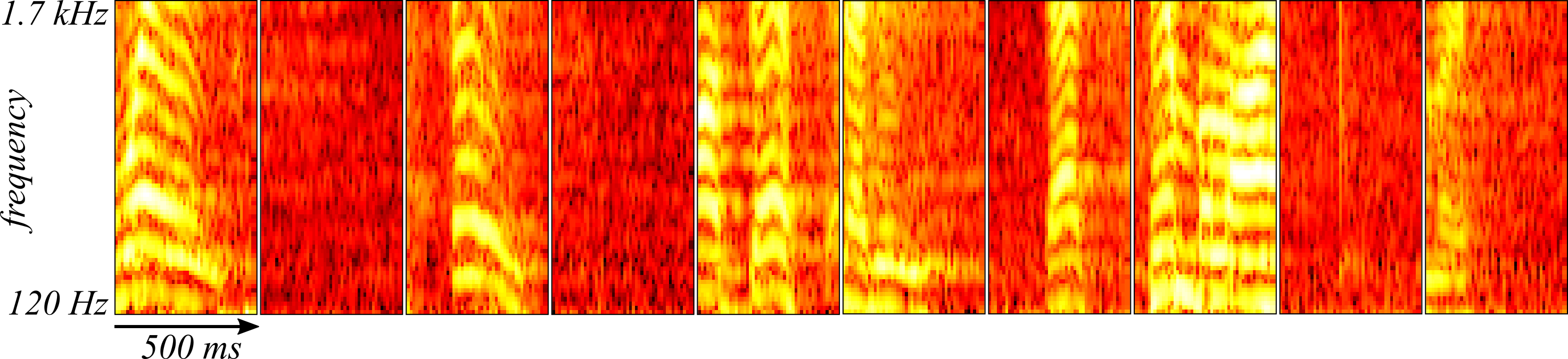
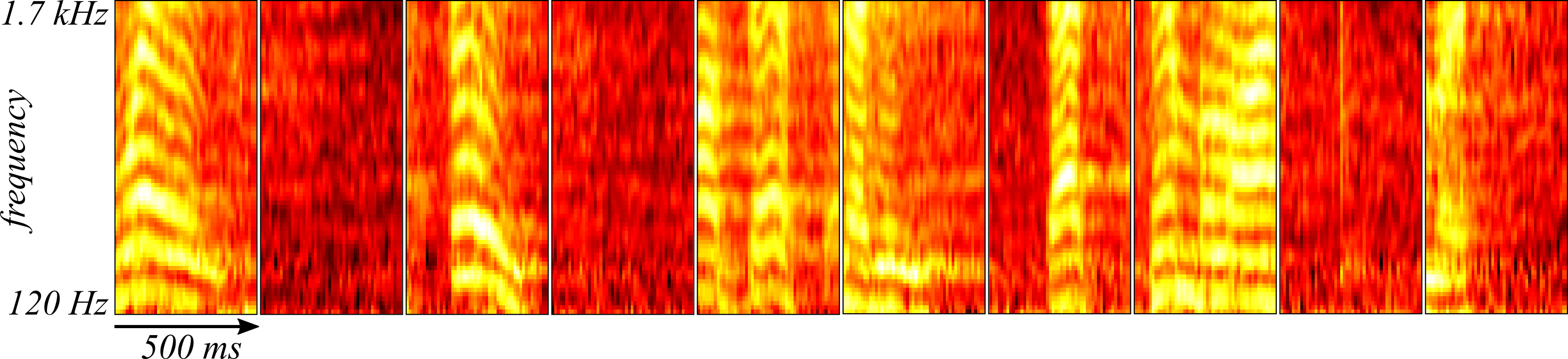
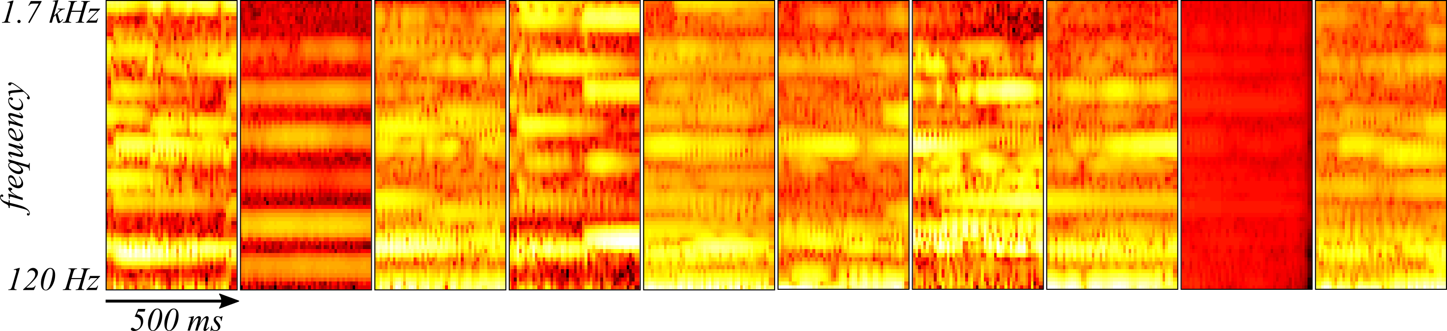
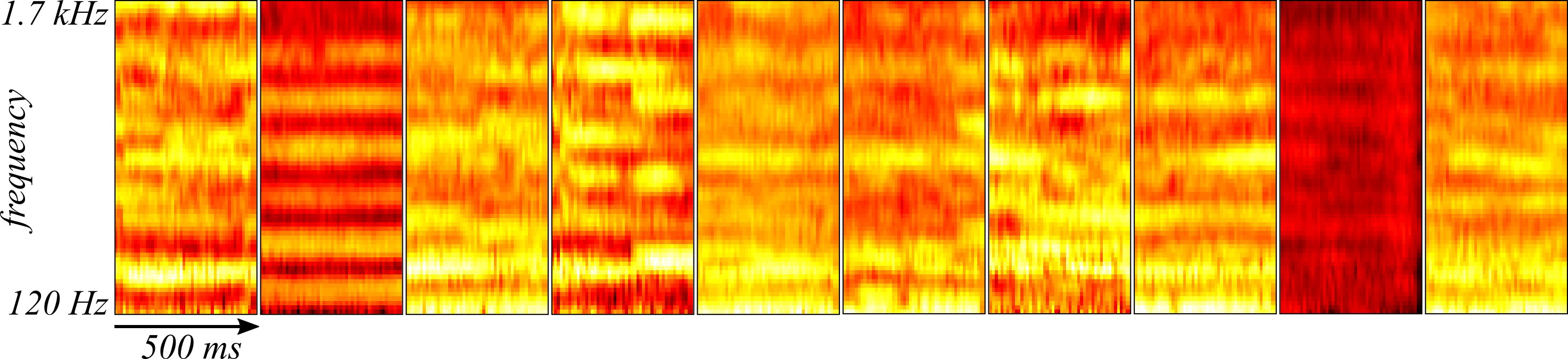
Let' take a look at the results. In Figure 2, ten random samples are drawn from the training set and plotted. These can be compared to the reconstructions by the convolutional autoencoder in Figure 3 (using the anonymous function predict from the above code) where the reconstruction appears to do quite well at recovering a smoothed version of the samples.
Using the convolutional autoencoder to compress the size of the data set can be done by defining different parts of the autoencoder as an encoder and decoder. It would make sense, then, to save outputs of the smallest layer of the network and treat subsequent layers in the flow of information as the network decoder. In this simple case, the encoder would be the convolution layer since it can describe the data in terms of sets of the outputs of the fifty units and the array patches which would require quite a lot less disc space than the 3600 dimensional spectrogram samples.
The optimized convolutional autoencoder was also tested on the reserved cross-validation samples taken from the end of the recording. Ten randomly sampled spectrograms from the cross-validation set are shown in Figure 4 and the reconstructions are found in Figure 5.
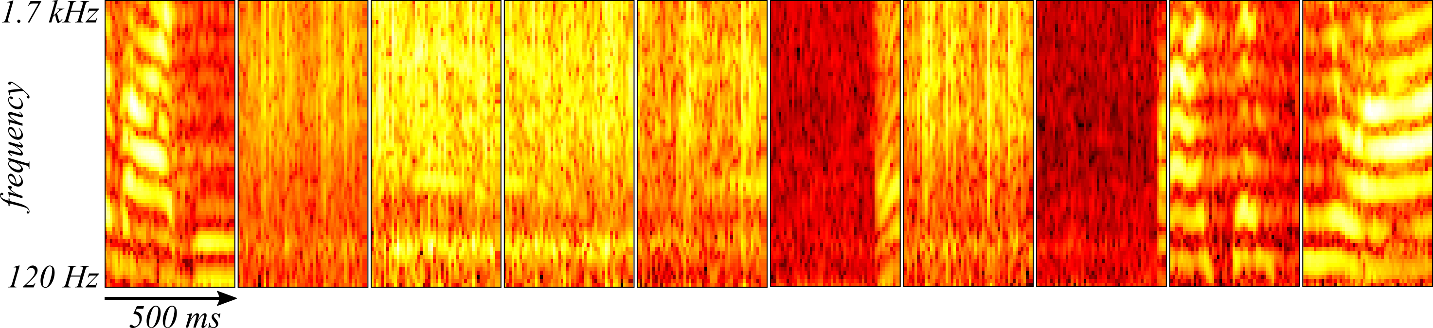
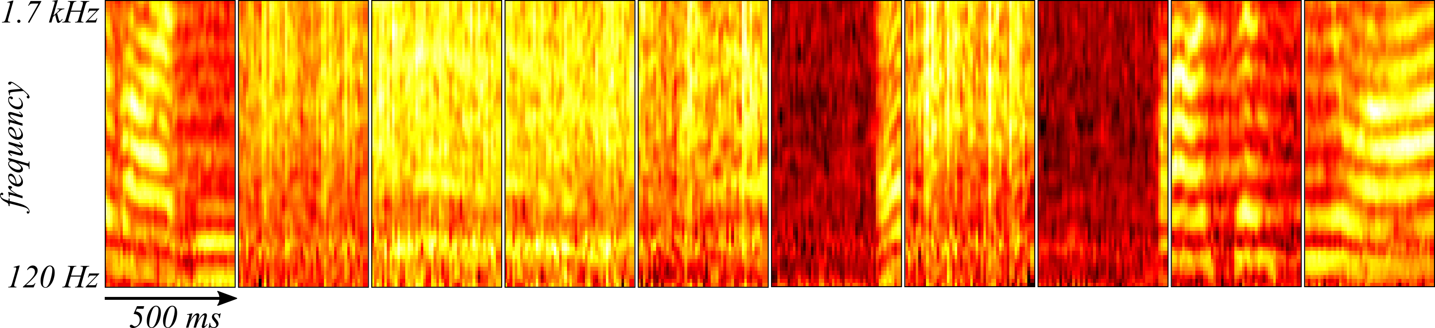
The convolutional autoencoder appears to be doing just as well at reconstructing the spectrograms drawn from the cross-validation set.
Could these results indicate that the convolutional autoencoder is uncovering something unique about President Kennedy's way of speaking? To test this idea, Johann Sebastien Bach's "The Art of Fugue" performed by Mehmet Okonsar with each movement played on either an organ or harpsichord was subjected to the same analysis as above except the spectrogram was scaled by the mean and standard deviation of President Kennedy's speech and the weights were not re-optimized. Ten randomly sampled spectrograms from the Art of Fugue appear in Figure 6 while their reconstructions with the convolutional autoencoder appear in Figure 7.
The reliability of the convolutional autoencoder in reconstructing Bach's "The Art of Fugue" despite its substantial differences from human speech suggest that the convolutional autoencoder is learning something more general about the histograms that is not unique to President Kennedy's speech. Instead, the convolutional autoencoder is likely learning either a smoothing or interpolation operation of the spectrograms.
Though it was not done in this example, one could also reconstruct the audio in amplitude vs. time space provided one keeps the phase information from the spectrograms by using the function angle().