The interior-point method is designed to find feasible local minimizers of optimization problems of the form

where \( \mathbf{x} \) is a vector of weights, \(f(\mathbf{x})\) is a scalar objective function, \(\mathbf{g}(\mathbf{x})\) is a vector of inequality constraints, and \(\mathbf{h}(\mathbf{x})\) is a vector of equality constraints.

If this is a constrained optimization problem, the usual unconstrained optimization algorithms will not maintain feasibility (i.e. satisfy the constraints) unless a particularly convenient initialization is chosen (and the minimum does not lie on a boundary of the feasible region) or a penalty function is used to promote feasibility (e.g. the \( \ell_2 \)-norm of the constraints). The significant caveat of the latter remedy is that the strength of this penalty function would need to go to infinity (or at least a machine approximation to infinity) to enforce feasibility near the boundary of the feasible region. On the other hand, constrained optimization methods like the simplex method are inadequate because the problem is (possibly) nonlinear. Thus, there is a need for a solver that can make guarantees about feasibility while also converging to a feasible local minimizer. Furthermore, it is desireable to have an infeasible algorithm that can converge to a feasible local minimizer despite initialization to an infeasible point. The interior-point method in the package pyipm seeks to achieve these ends.

The basics of the interior-point method include (i) transforming the constrained problem into an "unconstrained" problem via the method of Lagrange multipliers augmented by a barrier term, (ii) computing the gradient and Hessian (or approximating the Hessian with L-BFGS) of the Lagrangian with a simple modification to avoid saddle points on nonconvex problems, and (iii) a line search that minimizes a combined measure of sufficient decrease of the objective function and/or infeasibility. The latter two steps are then repeated ad nauseum until reaching a feasible local minimizer of the objective function where the Karush-Kuhn-Tucker (KKT) conditions are satisfied and the Hessian is positive semidefinite along feasible search directions (more specifically, the Hessian projected into the null space of the constraint Jacobians is positive semidefinite). For a more detailed account of this interior-point algorithm, see Chapter 19 of Nocedal & Wright, 2006. For background on the L-BFGS option, see Byrd, Lu, Nocedal, & Zhu, 1995.

Suppose, for whatever reason, we want to solve the following nonlinear program:

Figure 1: the objective function, \( f(x, y) \), plotted in \( x \) and \( y \) space. The infeasible region in overlayed in opaque red while the red lines correspond to the boundary of the feasible region defined by the constraint equations. Infeasible local minima are marked with cyan crosses while the lone feasible local minimum is marked with a green circle.

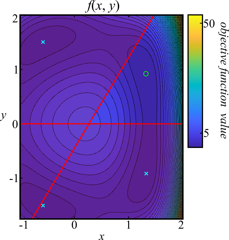
This problem is not easy to solve analytically (if at all) but it may be useful to approximate a solution numerically. We can solve this problem using the python package pyipm with the script outlined step-by-step in the following. The first step is to import the necessary dependencies (which need to installed if they are not already).

import numpy as np
import aesara
import aesara.tensor as T
import pyipm

The dependencies include NumPy (here aliased by np), the machine learning framework Aesara (a fork of the late, great, but now unmaintained, Theano), and pyipm. For brevity, it is convenient to also alias Aesara's tensor submodule as T. Next, a Aesara tensor variable definition is assigned to x which will symbolically represent both independent variables, \( x \) and \( y \), where x[0] \( \equiv x \) and x[1] \( \equiv y \). Symbolic expressions are then defined for the objective function and the inequality constraints in terms of the tensor variable x. The inequality constraints must be reformulated to be greater than or equal to zero; e.g. \( \frac{5}{3}x - y - \frac{9}{20} \geq 0 \).

# vector containing the independent variables x and y
x = T.vector("x")

# the objective function, f(x,y)
f = (1.0 + x[0] - x[0]**3)**2 + (1.61 - T.sqrt(T.sum(x**2)))**2 * (1.61 + T.sqrt(T.sum(x**2)))**2

# inequality constraints
ci = T.zeros((2,))
ci = T.set_subtensor(ci[0], 1.6667*x[0] - x[1] - 0.45)
ci = T.set_subtensor(ci[1], x[1])	

Note that the expressions for the objective function and constraints use the aesara.tensor variants of familiar NumPy functions. Care must be taken to use these instead of the NumPy equivalents or else errors will be encountered. It is also worth noting that, since these are expressions and not functions, that these cannot be evaluated without being compiled first (compilation functions give Aesara some of its speed). It will not be necessary for us to compile these functions, however, since pyipm does this for us internally. Furthermore, it is unnecessary to write expressions for the gradient and Hessian (if being computed) since pyipm will use Aesara's automatic differentiation functionality to generate and compile these expressions (though, in some cases, it may be possible to write a more efficient expression on your own; for instance, the Hessian for logistic regression was found to be much faster when I wrote own expression for the Hessian).

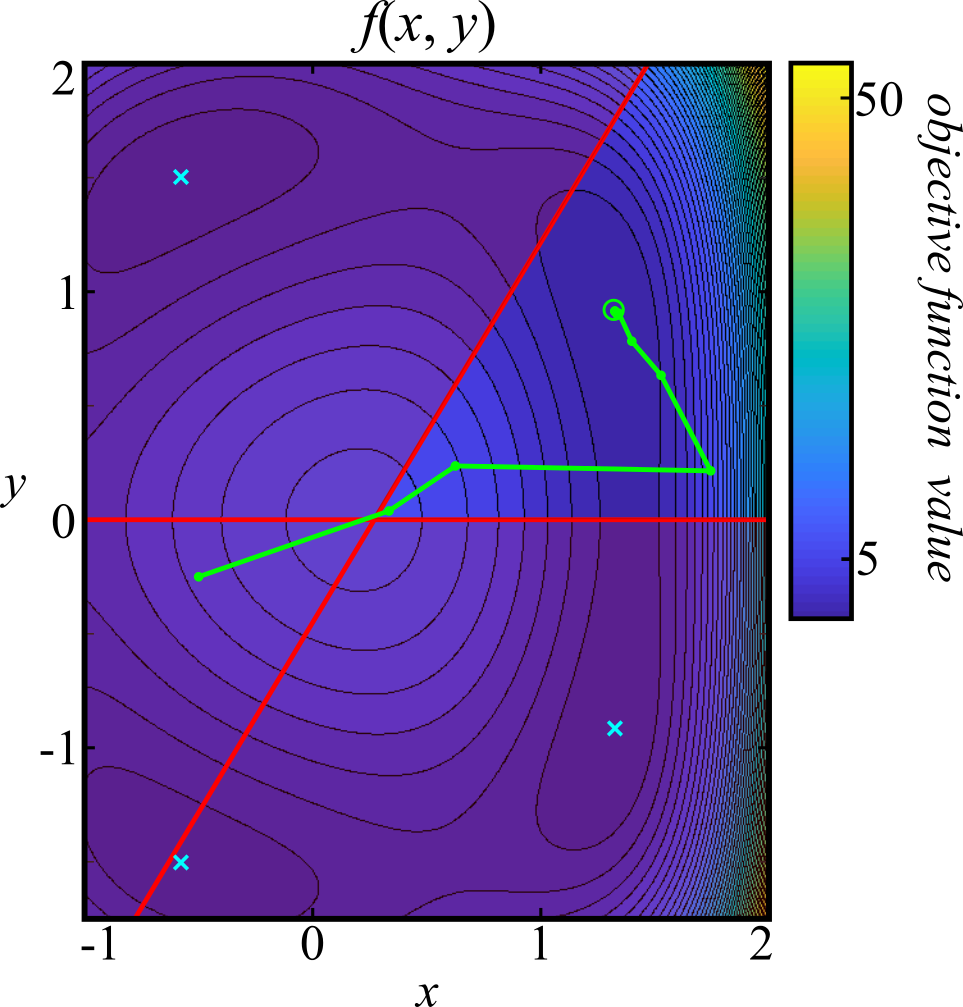
Before setting up the solver, an initialization of the independent variables is chosen. Usually, one may initialize them to random numbers (e.g. x0 = np.random.randn(2,)). However, for the sake of illustration, a specific infeasible choice is made to show that the solver will (i) find the feasible region and (ii) converge the feasible local minimum. An extra challenge was provided by initializing to a point where the gradient of the objective function clearly points away from the feasible region.

# initialization of the independent variables
x0 = np.array([-0.5, -0.25])

# problem initialization
problem = pyipm.IPM(x0=x0, x_dev=x, f=f, ci=ci, lbfgs=False, verbosity=2)

# Solve!
x, s, lda, fval, kkt = problem.solve()

The problem is then initialized by instantiating the class IPM from the pyipm package. By default, lbfgs is equal to False so one does not necessarily need to include that argument. If lbfgs is changed to a positive integer, then L-BFGS will be used with a memory equal to that integer used to approximate the Hessian. Finally, the pyipm.IPM.solve() function is called that compiles the Aesara expressions (if this has not been done already) and proceeds to search for a local minimizer until the KKT conditions are satisfied to user defined precision or the maximum number of user defined iterations are exceeded.

Solving our problem using the exact Hessian results in convergence to the point \(x = 1.3247\) and \(y = 0.9150\). Each iteration is plotted from initialization to convergence in Figure 2 where it can be seen that the interior-point method indeed escaped the infeasible region and converged to the feasible local minimum at the center of the green circle.

Figure 2: the interior-point method resists its desires for the lower-left infeasible local minimum and makes immediate and quick progress towards the feasible local minimizer in the upper-right. The green dots are iterations of the interior-point method (starting from the initialization at left) and are connected by a green line.

This example showed that pyipm can converge to a feasible local minimizer of a nonlinear and nonconvex constrained minimization problem. In the following examples, more problems will be solved to further demonstrate the abilities of this algorithm. It is worth pointing out here that there are, ultimately, limitations to interior-point methods. While convergence can be guaranteed to a local minimizer on unconstrained nonconvex objective functions, constraint satisfaction is a considerably more difficult problem. Convergence to a feasible point can only be guaranteed for affine equality constraints and convex inequality constraints and perhaps some functions that satisfy certain constraint qualifications. This means that nonlinear constraints are usually prone to converge to infeasible stationary points caused by the nonconvexity of the constraints. Nevertheless, one can always try multiple initializations until a feasible solution is found and that is a typical strategy used for problems where the constraints cannot be guarateed to be satisfied at a stationary point.