In this application, reinforcement learning will be used to teach a computer (the "agent") to play the game of tic-tac-toe. The problem will be approached in two different ways:

1. Tabular Q-learning.
2. Function approximation with policy gradients.

With a sufficient amount of experience in the form of repeated gameplay (or "episodes") and some tweaking of hyperparameters, both of these methods lead to the computer learning to play the game. In the case of tabular Q-learning, an interactive game is written in javascript where the user can participate in teaching the computer to play the game. With some hyperparameter tweaking, I was able to guide the policy gradients method to reach at least a 95% win rate against an opponent that makes valid moves with uniform probability.

Since this is a simple toy application of reinforcement learning rather than one that would be of particular interest to a seasoned practitioner of reinforcement learning, some effort is expended to give background and explanations on relevant theory and choices. For those who are unfamiliar with the topic, the goal of reinforcement learning is to teach an agent (e.g. a computer or robot) to perform a task optimally through actions that impact the state of the environment. While one could learn a policy through supervised learning on expert agents, learning from expert agents may lead to our agent learning a suboptimal policy. We would like to exceed the abilities of the experts if we can! Furthermore, experts may not be available in many tasks (though they are easy to come by in this toy example; e.g. you, probably!). This is what makes reinforcement learning a valuable approach to control problems.

What is tabular Q-learning? The "tabular" part refers to the usage of a lookup-table to store the expected return (i.e. the average future rewards) of a state, \( v(s) \), or state/action pair, \( q(s, a) \). The "Q-learning" part is a bit more complicated but focuses on learning \( q(s, a) \) which means for a given state \( s \) and action \( a \) the \( q(s, a) \) is the expected return. I will come to Q-learning shortly after taking a detour to discuss Monte Carlo and temporal-difference (TD) learning.

Suppose we have an episode of a game of tic-tac-toe as described in Fig. 1:

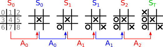
At each given state of the game, the agent could choose the optimal action given the current state from its state-action function, \( A_t = \mathrm{argmax}_a q(s=S_t, a) \), breaking any ties by, say, randomly choosing an action among the set of optimal actions. That is quite sensible, but how does one find the optimal action-value function? The first step is to define a reward function.

For each state/action pair, we can define a reward function that assesses the quality of the agent's choice and computes an immediate reward. The reward function should not depend on future or past states/actions, only the present state/action pair. Thus, an episode is composed of tuples \( (S_t, A_t, R_t) \) where \( R_t \) is the reward computed for the \( t \)th state/action pair. Note the difference between the reward and return for a given state/action pair. The reward is immediate while the return includes the immediate as well as the sum across all future (discounted) future rewards of the episode:

The discount factor is used to ensure that the return of continuous (non-episodic) scenarios converge. We can leave \( \gamma = 1 \) because tic-tac-toe is episodic and therefore the return will not diverge. Since we would like to avoid doing a tedious exercise in determining the reward of intermediate states, we use a simple terminal reward of \( R_{T - 1} = 1 \) if the agent wins, \( R_{T - 1} = -1 \) if the agent loses, and \( R_{T - 1} = 0 \) if the game is a draw. Note that in all definitions, only the states the agent sees are included in the sequence \( S_0, S_1, ..., S_{T-1} \) and not the states the opponent sees.

Before briefly summarizing a few learning algorithms, let's take a quick detour to talk about the agent's "policy". A policy is the function \( \pi(a|s) \) that gives the conditional probability of choosing an action given the current state. It seems obvious that one should choose the "greedy" policy, \( A_t = \mathrm{argmax}_a q(s=S_t, a) \), if \( q(s, a) \) is an optimal action-value function. What if the function is suboptimal, like when we first start learning the action-value function? Since we would like the agent to learn from experience, there is a danger that if the agent only chooses "greedy" actions it will fail to sufficiently explore and and improve the policy by choosing the alleged optimal action. This is where "epsilon-greedy" policies come into play where there is an \( \epsilon \) probability that the agent chooses a random action and a \( 1 - \epsilon \) probability the agent will greedily choose the action with the largest mean return. The policy function of an epsilon-greedy policy is therefore:

where \( \{ A \} \) is the set of all valid actions when in state \( s \).

For episodic cases, Monte Carlo learning of the action-value function is a fairly intuitive place to start. Monte Carlo learning is well suited to episodic cases because it requires that an episode terminate before it can be computed. For continuous scenarios, one can instead use temporal-difference (TD) methods. For the Monte Carlo algorithm, all we need to do is simply compute the return for each state/action pair at the end of each episode and then update the estimate of \( q(s, a) \), denoted by \( Q(s, a) \), by taking the average of the returns across episodes:

where \(m\) is the \(m\)th episode of \(M\) episodes and therefore \(G_n^{(m)}\) is the \(n\)th return of the \(m\)th episode and similarly for \(S_n^{(m)}\) for \(A_n^{(m)}\). The \(\delta_{x,y}\) is the Kronecker delta. Despite complicated appearances, this equation is simply an average of returns for a given state/action pair. This implementation of the average can be considerably simplified and made more scalable by keeping a running estimate of the average and updating that average using the latest return and a tally of the number of occurences of the state/action pair.

Temporal-difference (TD) methods, on the other hand, are better suited to continuous problems or long episodes where the agent can benefit from learning over the course of the episode instead of waiting for the distant termination of the episode. Unlike Monte Carlo learning, TD learning does not wait for future returns (at least in 1-step TD learning) but instead estimates the future return using the action-value function of the future state. The basic update rule for TD learning is:

where \( A_{n + 1} \) may be chosen using the policy \( \pi(a|s) \) and \( \alpha \in [0, 1] \) is the learning rate. This particular update algorithm is known as "SARSA" and there are some other variations like "expected SARSA" and Q-learning. The latter two are of particular value because they are "off-policy" learning methods.

"Off-policy" learning refers to the ability to learn from actions generated by a behavior policy different from the agent's own policy, like say the human opponent in tic-tac-toe, while "on-policy" learning means that the agent learns from actions only drawn from its own policy. The reason why this distinction is important is because some learning algorithms suffer from biases when the distribution of future rewards depends on decisions made by a policy other than the agent's own. Technically, Monte Carlo learning can perform off-policy learning using importance sampling. However, importance sampling has some undesirable qualities and is not practical in our tic-tac-toe example because it is not clear how to quantify the behavior policy of a human opponent.

We decide to apply Q-learning such that our agent can learn not only from its own actions but also from the actions of its human opponent. The update rule for Q-learning is:

where the only difference with SARSA is that the greedy future action is always taken. Therefore, when learning from an episode from the perspective of the human opponent, \( A_n \) is the action chosen by the human opponent while \( A_{n + 1} \) is chosen greedily according to the agent's estimated state-action function (in other words, the agent has a greedy policy). The behavior policy from the perpective of the agent's actions is epsilon-greedy while the agent's target policy is greedy.

Another method used to speed learning is to take advantage of the symmetry of the game. Tic-tac-toe exhibits rotational and mirror symmetry as shown in Fig. 2

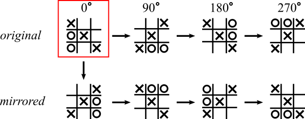
where the outcome of an episode will be the same regardless of whether the states are rotated or mirrored. Therefore, equivalent state/action pairs can be mapped to the same element of the lookup table for \( Q(s, a) \) greatly reducing the size of the state/action space (more on that below on function approximation).

A link to the demo of tabular Q-learning may be found here. The learning rate, discount factor, and epsilon probability of making a random valid move are adjustable in the provided fields.

Note that some of the code in this section is written in TensorFlow 2.0 and uses the default eager execution.

While tabular reinforcement learning is well suited to simple games like tic-tac-toe, there are a couple major issues with tabular reinforcement learning that make it impractical in many learning problems:

• Computer memory is finite. The number of possible state/action pairs will often exceed the memory limitations of computers.
• States/actions may be continuous. While binning states/actions may work in some cases, this may not be a desirable solution for others.

Of course, tic-tac-toe has discrete states and actions so we do not need to worry about the second point. What about the first point? It is easy to compute the total number of valid states in tic-tac-toe using recursion (it is a good idea to use memoization, as is done here, to speed up the calculation and avoid a potential stack overflow on ancient low memory machines):

import numpy as np

def check_win(state):
    # Check whether the current state is a winning state.
    s = state.reshape(3, 3)
    if np.any(np.prod(s == 1, axis=1)) or np.any(np.prod(s == 2, axis=1)):
        # Row win.
        return True
    elif np.any(np.prod(s == 1, axis=0)) or np.any(np.prod(s == 2, axis=0)):
        # Column win.
        return True
    elif np.prod(np.diag(s == 1)) or np.prod(np.diag(s == 2)):
        # Top-left to bottom-right diagonal win.
        return True
    elif np.prod(np.diag(s[:, ::-1] == 1)) or np.prod(np.diag(s[:, ::-1]) == 2):
        # Top-right to bottom-left diagonal win.
        return True
    else:
        # Non-win state.
        return False

def valid_actions(state):
    # Return a numpy list of valid actions given
    # the current state.
    if check_win(state):
        # This is a terminal state, return empty
        # actions list.
        return np.array([])
    else:
        # This is possibly a non-terminal state,
        # return any valid action indices.
        return np.where(state.ravel() == 0)[0]

def check_sym(state, state_set):
    # Check whether a symmetrically equivalent
    # state exists (subject to mirror and
    # rotation symmetries) and return key.
    s = state.reshape(3, 3)
    # Check rotations.
    for i in range(1, 4):
        key = tuple(np.rot90(s, i).ravel().tolist())
        if key in state_set:
            return True, key
    # Mirror across vertical axis and rotate.
    s = state.reshape(3, 3)[:, ::-1]
    for i in range(0, 4):
        key = tuple(np.rot90(s, i).ravel().tolist())
        if key in state_set:
            return True, key
    # Symmetric state not found.
    return False, tuple(state.tolist())

def num_states(allow_sym=True):
    # allow_sym when True means that all states are
    # counted while False counts only states unique to
    # mirror and rotation symmetry operations.
    
    # Declare hash table of all possible states.
    state_set = set()
    
    def recurse(state=None):
        
        if allow_sym:
            key = tuple(state.tolist())
        else:
            _, key = check_sym(state, state_set)
        if key in state_set:
            # This state has been seen before;
            # no need to explore this branch further.
            return
        
        # State has not been seen before, add it to
        # the hash table.
        state_set.add(key)
        
        # Get the indices of valid actions from the
        # current state. Terminal states return
        # no valid actions.
        actions = valid_actions(state)
        if len(actions) == 0:
            # Current state is full; this is a terminal
            # state and there are no valid actions.
            return
        else:
            if np.sum(state == 1) > np.sum(state == 2):
                # It is player "O"'s turn (player 2).
                turn = 2
            else:
                # It is player "X"'s turn (player 1).
                turn = 1
            for a in actions:
                # Evaluate all successor states.
                snext = np.copy(state)
                snext[a] = turn
                recurse(snext)
            return
        
    # Find all valid states.
    recurse(np.array([0] * 9))
    return state_set

If we do not merge states with rotational/mirror symmetry, running num_states(allow_sym=True) will reveal that there are 5,478 valid states (technically it is less than this because terminal states are included in the count but not in \( v(s) \)), the state-value function. If we merge symmetric states by running num_states(allow_sym=False), this number is reduced to 765 unique valid states. Storing up to \( 5,478 \times 8 \text{ bytes} = 43.8 \text{ kilobytes} \) of 64-bit floats is well below the memory limits of modern computers. Thus, tabular reinforcement learing is indeed well suited to tic-tac-toe. Although function approximation is not necessary, let's go ahead and do it anyway to demonstrate a specific form of function approximation known as "policy gradients".

Unlike the algorithms mentioned in the tabular reinforcement learning section which focused on learning an estimated action-value function, \( Q(s, a) \), policy gradients focus on directly learning an approximate policy function \( \hat{\pi}(a|s) \approx \pi(a|s) \). To be clear, function approximation is not restricted to policy gradients. One can also apply function approximation to learn \( Q(s, a) \) like in deep Q-learning. Although, function approximation of \( Q(s, a) \) has been shown to have stability issues and that is why we are going to focus on policy gradients here. What exactly is meant by function approximation? Function approximation means that we create a model that takes a state \( s \) as input and outputs a probability for each \( a \) that approximately replicates the behavior of the policy \( \pi(a|s) \) from estimating a tabular \( Q(s, a) \) without requiring the potentially large amounts of storage required. The policy can be approximated using models like logistic regression, neural networks, or other classifiers. In our case, we will be using a full-connected (dense) feed-forward neural network with residual connections similar to the one shown in Fig. 3.

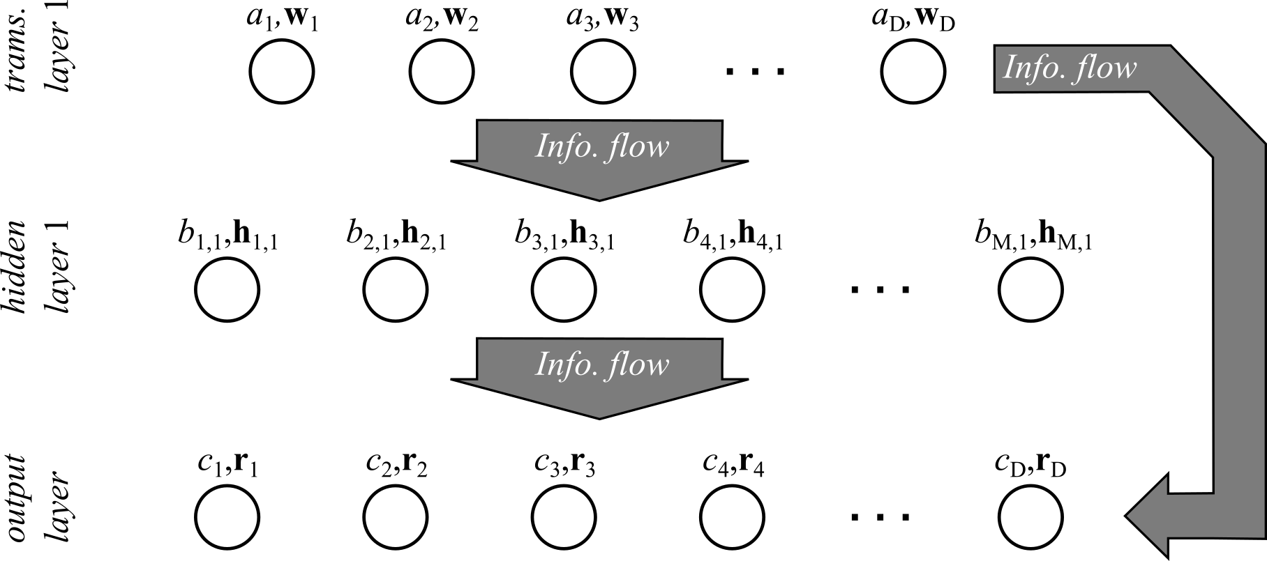
The weights of the network are initialized using Xavier initialization (Glorot normal initializer) and the biases are initially drawn from a uniform distribution in \( [0, 1] \). The initialization of the policy network parameters may be found in the __init__() method of the class ApproxPolicy. The method model() takes in a state \( s \) and evaluates the neural network returning the 9-dimensional output vector corresponding to \( \hat{\pi}(a|s) \) where the input and output are indexed as shown in the left-most board of Fig. 1 (however, model() accepts an arbitrarily shaped state and then unrolls it into a vector).

How do we go about training the policy network? There will be three different algorithms implemented that may be interchanged to the train the agent's policy all based on the policy improvement theorem. Since the optimal policy is the policy that maximizes the expected return, our goal should be to optimize our policy such that we maximize the state-value function \( v(s) \) for all states \( s \). The state value function may be written as \( v(s) = \sum_a q(s, a) \pi(a|s) \). The gradient of the value function can be computed as follows. More detail is provided on this derivation than others because there are few derivations of the policy gradient theorem that include discounting (at least that I had found at the time of writing this).

The result is a recursive function of the state-value function. Define \( \phi(s) = \sum_a q(s, a) \boldsymbol{\nabla} \pi(a|s) \) and \( P(s \rightarrow s', k) \) as the probability of transitioning from state \( s \) to \( s' \) in \( k \) steps where the following holds:

The gradient may be expanded in terms of \( \phi(s) \) and \( P(s \rightarrow s', k) \):

which is the final result. All we need to do to approximate this quantity is generate episodes, sampling actions from the policy \( \hat{\pi}(a|s) \) and sampling \( s' \) at step \( t \) from the \( t \)th step of the episodes. Based on this result, the implemented learning algorithms are:

1. REINFORCE,
2. REINFORCE with baseline,
3. and Actor-Critic.

where REINFORCE with baseline extends REINFORCE and Actor-Critic extends REINFORCE with baseline to online learning.

REINFORCE, the simplest of the three, is a straight-forward application of the above result where we recognize that \( q(S_t, A_t) = \mathbb{E}(G_t|S_t, A_t) \) and therefore we can replace \( q(S_t, A_t) \) with the sampled return \( G_t \). The stochastic gradient ascent update rule is:

following the conclusion of each episode where \( \alpha \) is a non-negative learning rate and \( T \) is used instead of \( \infty \) because this is an episodic problem (the sum is not always included in this definition but I included it because it seems we become slightly off-policy if we do not batch the weights; probably does not matter much though). The REINFORCE algorithm is implemented in the update_reinforce() method of ApproxPolicy where the baseline argument should be a function that simply returns zero.

REINFORCE with baseline allows for the addition of an arbitrary baseline function (so long as the baseline is not a function of the action) which can be used to reduce the variance of the updates while still being consistent with the policy gradient theorem. The update rule for REINFORCE with baseline is:

where \( b(s) \) is a baseline function. REINFORCE with baseline is implemented also using update_reinforce() but with the baseline parameter filled by a function taking in a state \( s \) and returning a scalar value for the baseline. A common choice for the baseline function is to use an estimate of the state-value function, \( V(s) \). In the case of tic-tac-toe, we can of course compute \( V(s) \) using tabular reinforcement learning as is done in the (poorly named) class ExactValue. Assuming we are simulating a case where the number of states is too large to fit into memory, an approximate state-value function may be estimated instead using a linear model as in ApproxValue. If we go the approximate state-value function route, the update rule for the coefficients of the value function is:

where \( \boldsymbol{\rho} \) is a vector of the linear model coefficients of the value function, \( \beta \) is a separate non-negative learning rate for the value function, and \( V(S_t, \boldsymbol{\rho}) \) is the value function used as a baseline function. This is a semi-gradient update rule which is proven to converge for linear models but has not been proven to do so for more sophisticated models. Note that while a bad function approximation of the value function could lead to high variance, REINFORCE with baseline should still asymptotically converge to an optimal approximate policy.

Actor-critic is similar to temporal-difference (TD) learning discussed above in the tabular reinforment learning section. Actor-critic learning is advantageous in cases where online learning may be helpful/necessary for the same reasons as TD learning. Actor-critic estimates the n-step return by bootstrapping the update rule from REINFORCE with baseline with following approximation:

Being an online method, Actor-critic learning does not require waiting until the the end of the episode to start learning but may start once \( n \) steps of the episode have taken place. The learning update for n-step actor-critic may be found in the update_actor_critic() method of the class ApproxPolicy.

To speed up learning, much like in the tabular setting, it would be nice to take advantage of the symmetry of the game. However, we are not going to put any explicit constraints on the model to do so (like in the tabular case) but instead augment the dataset by training on the same episode subjected to rotation and mirroring operations as in Fig. 2. We can instead handle off-policy learning via importance sampling introducing a behavior policy \( \pi_b(a|s) \). If \( \phi \) represents a function that returns a state equivalent to rotating the tic-tac-toe board 90 degrees clockwise and \( \omega \) is a function that returns a state that mirrors the board across the vertical axis, then \( s' = \phi(\omega(s)) \) would produce a state that is equivalent to the original state except mirrored across the vertical axis and then rotated by 90 degrees clockwise. In this case, the behavior policy is the result of applying the exact same operations to the approximate policy as to the state/action pairs. For example, if the augmented sample has \( s' = \phi(\omega(s)) \) and \( a' = \phi(\omega(a)) \), the behavior policy would be output would be \( \pi_b(a|s') = \phi(\omega(\hat{\pi}(a|s,\boldsymbol{\theta}))) \) while the target policy distribution would be simply \( \hat{\pi}(a|s',\boldsymbol{\theta}) \). We can attempt derive an equivalent expected state-value with sampling over the behavior policy as follows:

where \( P_b(s \rightarrow s', t) \) is the probability of transitioning from \( s \) to \( s' \) under the behavior policy. This result seems reasonable as we simply reweight by the probability of entering the state \( s' \) and taking the action \( a \). However, there are a couple issues:

1. computing the transition probabilities is impractical because it would require computing the probabilities of all actions in each of the intermediate states between \( s \) and \( s' \) and
2. sampling from the behavior policy to estimate \( q(s', a) \approx G_t \) in the Monte Carlo case would lead to estimating the target policy return with the behavior policy return.

A way to handle the first issue is to drop the transition probability factor from the expectation:

which can still achieve an optimal policy (though it adds additional local maxima, some which may be suboptimal)[2]. The second issue may be resolved by reweighting all of the future rewards by the relative probability of the sequence of states/actions between the target and behavior policy:

which is a general solution for both n-step actor critic and REINFORCE algorithms.