Maximum noise entropy (MNE) models are models constructed using the principle of maximum entropy with the goal of limiting bias towards unexplored regions of feature space. Intuitively, bias is defined in the sense of Occam's razor, where the principle of maximum entropy attempts to find a model with little structure other than that imposed by evidence/constraints. For example, if a loaded die is known to land on six with a probability of 1/3 but it is unknown what the individual probabilities are of landing on one through five, the simplest model would be to assume that the die lands on one through five with equal probability in the absence of further evidence. Coming up with a more complicated model that assigns a more favorable probability to landing on one, for example, could be seen as a biased model.

Now, let's take a look at the math of MNE. The mutual information between between some feature vector (independent variables), \( \mathbf{s} \), and the scalar response (dependent variable), \( y \), is \( I(y, \mathbf{s}) = H_\mathrm{resp}(y) - H_\mathrm{noise}(y, \mathbf{s}) \) represented here by the difference between a response and noise entropy. A minimally biased conditional probability distribution, \( P(y|\mathbf{s}) \), can then be achieved by minimizing the mutual information between \( y \) and \( \mathbf{s} \). Since \( H_\mathrm{resp} \) does not depend on \( \mathbf{s} \), it is a constant. Therefore, minimizing the mutual information is equivalent to maximizing the noise entropy.

From a computational point of view, a neuron can be viewed as a binary classifier where a neural response (a "spike") is represented by \( y = 1 \) while silence is \( y = 0 \). For sensory neurons, the feature space is composed of external stimuli (like images for vision neurons and spectrograms for auditory neurons). To limit bias being imposed on the function that relates the probability of a spike to stimuli, only empirical constraints are set on \( P(y|\mathbf{s}) \) in the form of spike-weighted moments of the stimulus space (e.g. \( \langle y \rangle \), \( \langle y \mathbf{s} \rangle \), \( \langle y \mathbf{ss}^\mathrm{T} \rangle \), ...). For a classifier, the maximum entropy probability distribution of a spike is

which as analytic solution to the primal problem while the weights \(a\), \(\mathbf{h}\), \(\mathbf{J}\), ... are the Lagrange multipliers that need to be optimized (and form the dual problem). The argument, \(z(\mathbf{s})\) is a polynomial. First-order and second-order truncate \( z(\mathbf{s}) \) to first (\(a + \mathbf{h}^\mathrm{T} \mathbf{s} \)) or second-order (\(a + \mathbf{h}^\mathrm{T} \mathbf{s} + \mathbf{s}^\mathrm{T} \mathbf{J} \mathbf{s} \)) and these are the models that are optimized in the C program cmne. The weights are optimized by maximizing the log-likelihood objective function. This optimization is convex and early stopping is used to limit overfitting.

The cmne code was used in the publication Kaardal, Theunissen, & Sharpee, 2017.

One of the difficulties in characterizing receptive fields of neurons, and more generally dimensionality reduction, is that correlated datasets can lead to biased characterizations of the relevant subspace. For this example, we are going to take a look at this issue by comparing a linear method called spike-triggered covariance (STC) to second-order MNE and show that MNE better captures the receptive field of a synthetic sensory neuron stimulated by correlated Gaussian stimuli.

The stimuli are two-dimensional and can be interpreted as being either images or spectrograms for either vision or auditory neurons, respectively. The individual pixels of the stimuli are Gaussian distributed and correlated with nearby pixels. The multivariate Gaussian distribution the stimuli are drawn from has covariance kernel

where \( \mathbf{r}^\mathrm{T} = \left[ x, \, y \right] \) are the coordinates of the image/spectrogram, \( \sigma_1 = \sigma_2 \) is the correlation distance, and \( \mathrm{diag}(\cdot) \) is a function that transforms a vector into a diagonal matrix. In total, \( N_\mathrm{samp} = 100000 \) stimuli were generated and each stimulus was a \( 16 \times 16 \) square of pixels unrolled into \( D = 256 \) dimensional vectors.

The ground truth receptive field of the synthetic neuron is spanned by the six components shown in Figure 1.

Figure 1: the six ground truth receptive field components of the synthetic neuron.

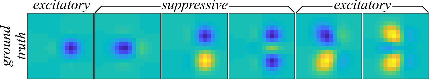
These receptive fields are formed from the eigenvectors of a sum of the outer products of six non-isotropic two-dimensional Gaussians. The suppressive components have negative eigenvalues which corresponds to a decrease in the neural response to positive amplitudes in the stimuli while the excitatory components increase the neural response to positive stimulus amplitudes. The set of ground truth receptive field components, \( \Omega_\mathrm{GT} = \big\{ \mathbf{\omega}_\mathrm{GT}^{(k)} | \text{ for all } k \in \{ 1, \cdots, 6 \} \big\} \), are combined into the outer product matrix \( \mathbf{J}_\mathrm{GT} = \sum_{k=1}^6 \lambda_\mathrm{GT}^{(k)} \mathbf{\omega}_\mathrm{GT}^{(k)} \mathbf{\omega}_\mathrm{GT}^{(k)\mathrm{T}} \) where \( \lambda_\mathrm{GT}^{(k)} \) are the eigenvalues of each component. With the matrix \( \mathbf{J}_\mathrm{GT} \), the spiking probability is computed across all stimuli using the second-order MNE nonlinearity from above, \( P(y=1|\mathbf{s}) \), and the threshold, \( a_\mathrm{GT} \), is adjusted until the mean spiking rate is around \( 0.25 \) spikes per stimulus sample. The linear component, \( \mathbf{h}_\mathrm{GT} \), was set to zero. The responses for all \( t \in \{ 1, \cdots, N_\mathrm{samp} \} \) were binarized by comparing a uniform random number, \( \xi_t \in \left[0, \, 1 \right] \), to \( P(y=1|\mathbf{s}_t) \) of the \(t\)th stimulus where \( \xi_t \leq P(y=1|\mathbf{s}_t) \) leads to the response \( y_t = 1 \) and otherwise \( y_t = 0 \).

Now, we move on to trying comparing the ability of second-order MNE and STC to recover the components in Figure 1. STC recovers the receptive field through eigendecomposition of the difference between two covariance matrices:

where \( N_\mathrm{spk} = \sum_{t=1}^\mathrm{Nsamp} y_t \). Through eigendecomposition of \( \mathbf{C}_\mathrm{STC} \) into its eigenvectors and eigenvalues, \( \mathbf{C}_\mathrm{STC} = \mathbf{\Omega}_\mathrm{STC} \mathbf{\Lambda}_\mathrm{STC} \mathbf{\Omega}_\mathrm{STC}^\mathrm{T} \), we hopefully find that the components recovered from the six largest magnitude positive or negative eigenvalues/eigenvectors will be a good approximation to the subspace of stimulus space spanned by the ground truth receptive field. Since STC is a model independent method (i.e. used alone, it does not provide a recipe for making predictions), we can instead compare the subpsace overlap of the ground truth and STC receptive fields using the overlap metric from Fitzgerald & Sharpee, 2011:

where \( D \) is the number of rows in \( \mathbf{C}_\mathrm{STC} \). The overlap metric is bounded between zero and one where one indicates that the two subpaces completely overlap while zero means the subspaces are disjoint. Using the overlap metric, the subspace overlap of the recovered receptive field via STC is \( \mathcal{O}(\mathbf{\Omega}_\mathrm{STC}, \mathbf{\Omega}_\mathrm{GT}) = 0.003 \) (where \( \mathbf{\Omega}_\mathrm{GT} \) are the six eigenvectors of \( \mathbf{J}_\mathrm{GT} \)). Despite the similarities between the STC-recovered components (Figure 2 bottom) and the ground truth, STC performs rather poorly by this quantitative measure and describes a subspace almost entirely disjoint from the ground truth. If we take a look at Figure 2, we can see that there is indeed an apparent distortion of the receptive field where the amplitudes are not as sharply localized in the two-dimensional space.

Figure 2: the six ground truth receptive field components of the synthetic neuron (top) and the receptive field recovered via STC (bottom). The STC components exhibit substantial distortion.

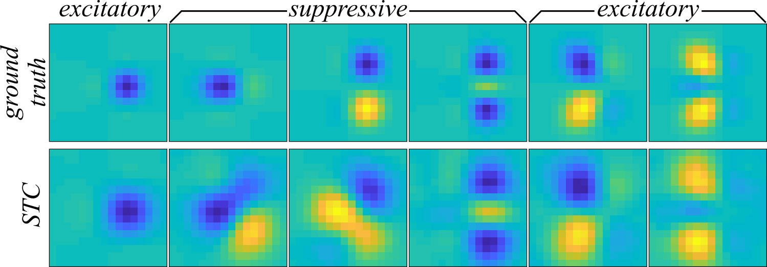
The reason why STC fails to recover the receptive field is because STC provides a biased estimate when the stimuli are not drawn from an uncorrelated Gaussian distribution. Since the stimuli in this example were drawn from a correlated Gaussian distribution, this bias is the most likely source of the observed distortion in Figure 2. MNE, on the other hand, is designed to be low-bias for generic distributions and is expected to perform better. For the second-order MNE fits, the cmne code was used. The second-order MNE models were trained on 70% of the data and cross-validated on 20% of the data for early stopping. Four different jackknives were computed with random samples drawn from the data set to form the training and cross-validation sets. The cmne code does this automatically by setting the variables train_fraction = 0.7, cv_fraction = 0.2, and Njack = 4 in the code cmne_blas.c. To perform second-order MNE, the variable rank must be assigned to -1 which automatically determines the size of the matrix from the dataset. The remaining settings were left unchanged. After compiling, the code is run by typing

./cmne_blas stimulus_filename response_filename output_directory output_label

into a terminal (assuming one is in the same folder as the code). The command line arguments are fairly self-explanatory, corresponding to file input and output information. The output of the code will appear in the folder "output_directory" and will be in a binary format. The files that begins with "params" contain the vector \( \mathbf{x}^\mathrm{T} = \left[ a, \, \mathbf{h}^\mathrm{T}, \, \mathbf{J}(:)^\mathrm{T} \right] \) (where \( \mathbf{J}(:) \) indicates that matrix \( \mathbf{J} \) is unrolled into a column vector) from each jackknife, denoted by the suffixes "j0", "j1", "j2", and "j3" for the first through fourth jackknives, respectively.

After the running the cmne code, the \( \mathbf{J} \) matrices from each of the jackknives was decomposed into eigenvalues and eigenvectors, \( \mathbf{J} = \mathbf{\Omega} \mathbf{\Lambda} \mathbf{\Omega}^\mathrm{T} \), and the three largest variance component positive and three largest variance negative components were recovered as an approximation to the receptive field. The components recovered by MNE are plotted in Figure 3 (bottom) and match the extent of the components much better than STC in Figure 2. On the other hand, the MNE components are substantially more noisy than the STC components, and the amount of noise corruption increases as the variance of the components decrease.

Figure 3: the six ground truth receptive field components of the synthetic neuron (top) and the receptive field recovered via second-order MNE (bottom). Though not necessarily obvious, the MNE components better recover the receptive field subspace compared to STC.

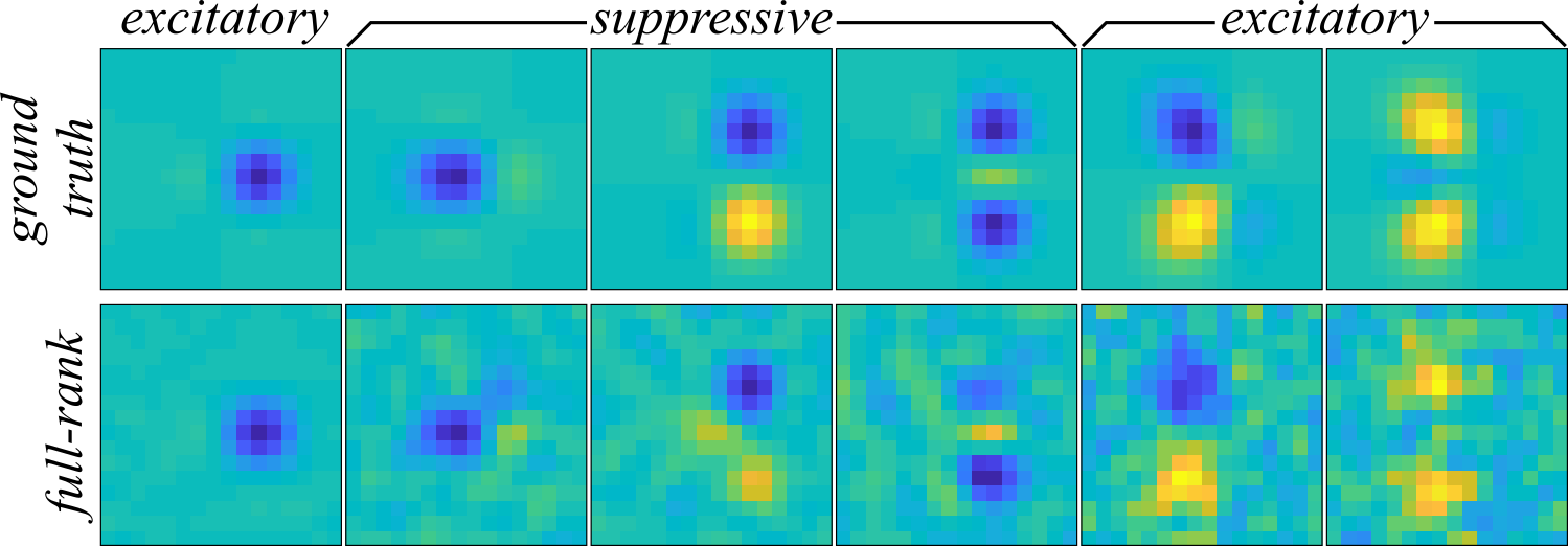
With an subspace overlap of \( \mathcal{O}(\mathbf{\Omega}, \mathbf{\Omega}_\mathrm{GT}) = 0.7 \pm 0.1 \) average across jackknives, the second-order MNE receptive field much better captures the receptive field than STC.

This example problem will be returned to when discussing the low-rank maximum noise entropy model. The low-rank maximum noise entropy example shows that further improvements can be made over the full-rank second-order MNE models on this synethic neuron.