For background on second-order maximum noise entropy (MNE) models, see the Maximum Noise Entropy method. This low-rank method is used to recover multicomponent receptive fields of sensory neurons when the feature space is poorly explored. The model is modified in two key ways. (i) The quadratic weights, the \( D \times D \) matrix \( \mathbf{J} \), are prefactorized before optimization via the bilinear factorization \( \mathbf{J} = \mathbf{UV}^\mathrm{T} \) where \( \mathbf{U} \) and \( \mathbf{V} \) are \( D \times r \) matrices. (ii) \( \mathbf{U} \) and \( \mathbf{V} \) are constrained to span the same range space such that \( \mathrm{rank}(\mathbf{J} + \mathbf{J}^\mathrm{T}) \leq r \). Further structure is imposed on \( \mathbf{J} \) through sparse penalization of the rank of \( \mathbf{J} \) with nuclear-norm regularization \(\ell_*(\mathbf{U}, \mathbf{V}) = \frac{1}{2} \left[ ||\mathbf{U}||_2^2 + ||\mathbf{V}||_2^2 \right] \). The penalized log-likelihood is then maximized subject to constraints that satisfy (ii) where cross-validation data can be used to set the regularization parameter(s). The nuclear-norm and explicit factorization of \( \mathbf{J} \) are based on the assumption that the dimensionality of a neuron's receptive field is less than the total dimensionality of the feature space. This is equivalent to saying the the meaningful dimensionality of the feature space is much less than the dimensionality of the feature space that describes all possible features.

Unlike (full-rank) second-order MNE, low-rank MNE is nonconvex. However, since the nuclear-norm regularization penalty function is convex, there is a threshold strength of the penalty function such that local maximum of the problem can be certified as a global maximum. This can be proven by showing that the solution to the low-rank MNE problem is equivalent to a convex relaxation of an equivalent (nonlinear) semidefinite program. This was shown in the appendices of Kaardal, Theunissen, & Sharpee, 2017 and is based off the work of Bach, Mairal, & Ponce, 2008 and Haeffele, Young, & Vidal, 2014. An algorithm is proposed that can solve for a "globally optimal approximation" to the receptive field by using the minimal amount of nuclear-norm regularization to reach the globally optimal regularization domain. The python package mner includes this algorithm as well as a locally optimal algorithm that uses Bayesian optimization to discover hyperparameter settings that lead to an MNE model with good generalization ability to novel data.

This method was published in Kaardal, Theunissen, & Sharpee, 2017.

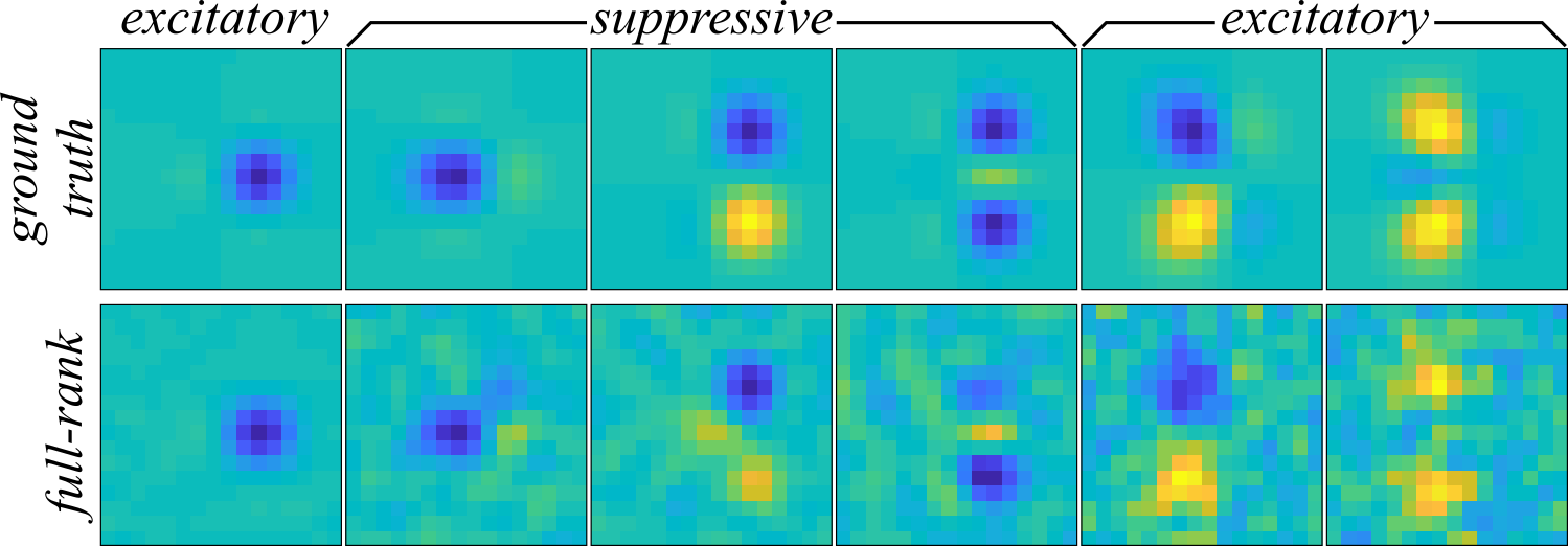
This example is a continuation of Example 1 from the maximum noise entropy project where a six component receptive field of a synthetic sensory neuron is recovered using STC and full-rank (second-order) MNE. It was found in that article that full-rank MNE was a better choice for recovering the receptive field compared to STC since the stimuli are drawn from a correlated Gaussian distribution. For more background on the problem, follow the link at the beginning of this paragraph. In this present example, low-rank MNE will be applied to gain further improvements over the full-rank MNE model in recovering the receptive fields of the synthetic sensory neuron.

The full-rank MNE model recovered the six component receptive field in Figure 1 (bottom) which appears to be corrupted by a correlated noise distribution in the lower variance components at right when compared to the ground truth (Figure 1 top).

Figure 1: the six ground truth receptive field components of the synthetic neuron (top) and the receptive field recovered via full-rank second-order MNE (bottom). The lower variance components at right appear to be increasingly corrupted by correlated noise.

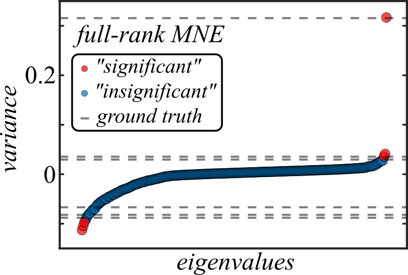
Furthermore, in Figure 2 one can see from the mean eigenvalue spectrum of \( \mathbf{J} \) that noise is actually a very large contributor to the overall variance of \( \mathbf{J} \), which may suggest that the model is still overfit even with early stopping (though early stopping certainly helps; without it, correlated noise comes to dominate the variance of \( \mathbf{J} \)).

Figure 2: eigenvalues of matrix \( \mathbf{J} \) obtained from full-rank MNE averaged across jackknives with the components from Figure 1 marked in red. Correlated noise makes a large contribution to the overall variance (blue). The gray dashed lines are the ground truth eigenvalues.

To improve upon these results by eliminating the noise corruption, the low-rank MNE method is used. The following goes through the steps of defining and optimizing low-rank MNE models to find a globally optimal approximation of the receptive field.

We can start by importing the necessary packages into our python script (give them aliases, if desired).

import numpy as np
import theano
import mner.optimizer
import mner.util.util
import mner.solvers.solvers
import mner.solvers.constraints
import mner.solvers.samplers
import sys

The low-rank MNE package, mner, does not automatically import subpackages so one must import needed subpackages and modules explicitly (similar to SciPy and unlike NumPy). Let's now prepare the data set for analysis. Like with the full-rank MNE models, the same four jackknives are fit where 70% of the samples are assigned to the training set (and 20% to cross-validation, though we do not use it here).

jack = 1             # jackknife to compute; 0 < jack <= njack
njack = 4            # total number of jackknives
train_fraction = 0.7 # fraction of samples in training set
cv_fraction = 0.2    # fraction of samples in the cross-validation set

# either construct or load from file the following variables...
# s: a numpy array sampling the ndim dimensional feature (stimulus) space with s.shape = (nsamp, ndim)
# y: is a numpy array of responses to the nsamp samples of feature space in s with y.shape = (nsamp,)

# feature scaling, if not already done (recommended, but not required)
s, s_avg, s_std = mner.util.util.zscore_features(s)

# generate Boolean indices for y and the rows of s defining the training set and circularly shift according to jack
trainset, cvset, testset, nshift = mner.util.util.generate_dataset_logical_indices(train_fraction, cv_fraction, nsamp, njack)
trainset, cvset, testset = mner.util.util.roll_dataset_logical_indices(trainset, cvset, testset, nshift, jack-1)

# store the Boolean indices in the datasets dictionary
datasets = {'trainset': trainset, 'cvset': cvset, 'testset': testset}

In the source code, which may be found here, the data is generated in the commented lines above; but that procedure is suppressed here because it is quite lengthy. The formatting choices made above will be important later, particularly the shape of the arrays "s" and "y" should follow the above convention and the "datasets" dictionary will be needed by the optimizer.

Next, we define the low-rank MNE problem we want to solve and how we would like to solve it. The following code will define a rank 6 \( \mathbf{J} \) matrix with up to three positive and three negative eigenvalues under the constraint that the positive variance components satisfy \( \mathbf{U} = \mathbf{V} \) and the negative variance components satisfy \( \mathbf{U} = -\mathbf{V} \).

# model parameters
rank = 6
cetype = ["UV-linear-insert"]
rtype = ["nuclear-norm"]

# if J is symmetrized using linear constraints, need to set signs of eigenvalues
csigns = np.array([1, -1]*(rank/2))

To apply these constraints, the variable cetype is set to the (list of the) string "UV-linear-insert" which will tell the optimizer to apply the constraints we want. Since the constraints are linear, this string also tells the optimizer to directly insert the constraints into the objective function rather than forming the Lagrangian. The variable rtype is assigned to the (list of the) string "nuclear-norm" that tells the optimizer to apply a nuclear-norm regularization penalty. The additional variable csigns must be defined when using either the "UV-linear" or "UV-linear-insert" constraints to tell the optimizer which columns of \( \mathbf{U} \) and \( \mathbf{V} \) have either a positive (1) or negative (-1) eigenvalue. Then, we choose a solver and the scaling of the log-likelihood objective function in the following bit of code.

# set scaling of the log-likelihood objective function (for each data set)
fscale = {"trainset": -1, "cvset": -1, "testset": -1}

# choose solver
solver = mner.solvers.solvers.LBFGSSolver

# fit parameters
factr = 1.0e7
lbfgs = 30

The dictionary fscale tells the optimizer how to scale the log-likelihood objective function with respect to each data set. By setting the value to a negative number, the optimizer will determine the number of samples in each data set and divide the log-likelihood portion of the objective function by the number of samples. The variable solver is assigned to a solver class (not an instance), in this case a class that wraps around fmin_lbfgs_b from scipy.optimize, a bound-constrained (or unconstrained) L-BFGS algorithm. The variables factr, that determines the convergence precision, and lbfgs, which is an integer length of stored objective gradient history, are passed to the solver by the optimizer.

Finally, we can search for a globally optimal approximation of the receptive field. The globally optimal approximator finds the minimal value of the nuclear-norm regularization parameter that leads to a globally optimal solution for the penalized objective empirically by minimizing a series of penalized objective functions for various values of the nuclear-norm regularization parameter. This suproblem is solved using the L-BFGS solver from the variable solver above. The following code shows the last steps of the script.

# globally optimal approximator
global_solver = mner.solvers.solvers.NNGlobalSearch

# instantiate the optimizer
opt = mner.optimizer.Optimizer(y, s, rank, cetype=cetype, rtype=rtype, solver=global_solver, datasets=datasets, 
                              fscale=fscale, csigns=csigns, lbfgs=lbfgs, precompile=True, compute_hess=False, 
                              verbosity=2, iprint=1, factr=factr, nn_global_search_solver=solver, 
                              nn_global_search_maxiter=100)

Here everything comes together. The globally optimal approximator class is assigned to global_solver and everything is passed into the optimizer class. A few new options appear at this point as well, including precompile, compute_hess, verbosity, and iprint. The variable precompile must be set to True because the L-BFGS code will not compile Theano expressions. The Hessian is not necessary for L-BFGS, so compute_hess = False. The variables verbosity and iprint determine the amount of screen output from the optimizer and the L-BFGS code, respectively (larger numbers = equal/more screen output). At last, the problem is solved, returning the optimal weight vector, x, and the final (penalized) objective functional value at x.

# solve!
x, ftrain = opt.optimize()

# split up and reformat weight vector
a, h, U, V = mner.util.util.vec_to_weights(x, ndim, rank)

# recover J
Jsym = np.dot(U, V.T)
Jsym = 0.5*(Jsym + Jsym.T)

The weight vector x is then split up into coefficients and the \( \mathbf{J} \) matrix, Jsym, is recovered. The receptive field can then be reconstructed through eigendecomposition of Jsym.

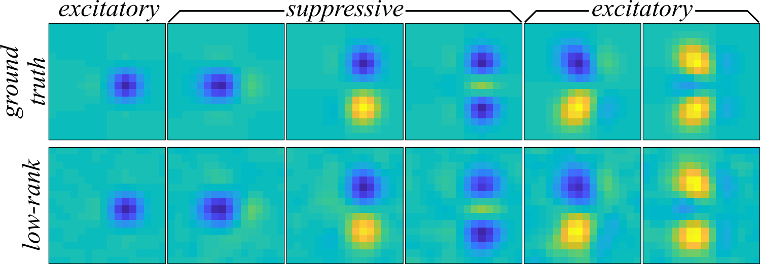
The receptive field components recovered with the low-rank MNE method's globally optimal approximation can be found in Figure 3. Compared to the full-rank MNE model, the components are much cleaner, exhibiting no apparent noise corruption. In fact, the low-rank MNE model recovers the receptive field nearly perfectly with a subspace overlap of \( \mathcal{O}(\mathbf{\Omega}, \mathbf{\Omega}_\mathrm{GT}) = 0.9861 \pm 0.0009\) average across jackknives (see here for a definition of the overlap metric). The subspace overlap is a statistically significant improvement over the full-rank MNE models where \( \mathcal{O}(\mathbf{\Omega}, \mathbf{\Omega}_\mathrm{GT}) = 0.7 \pm 0.1 \).

Figure 3: the six ground truth receptive field components of the synthetic neuron (top) and the receptive field recovered via low-rank second-order MNE (bottom). Note that the correlated noise from Figure 1 has disappeared.

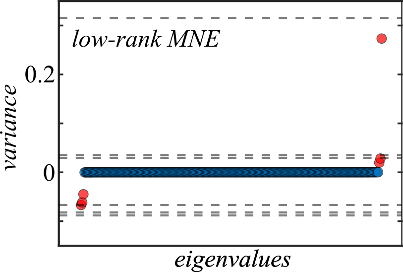
As expected, the variance of \( \mathbf{J} \) is entirely confined to the six significant components (Figure 4) instead of shared among a multitude of noisy eigenvalues like in Figure 2.

Figure 4: eigenvalues of matrix \( \mathbf{J} \) obtained from low-rank MNE averaged across jackknives with the components from Figure 1 marked in red. Note that eigenvalue is of the specified rank and the noise eigenvalues are all zero (blue). However, nuclear-norm regularization has led to some attentuation of the variance relative to the ground truth (gray dashed lines).

Of course, nuclear-norm regularization ends up attenuating the variance of the components in its effort to find a globally optimal approximation. Though it is not a substantial issue for this neuron, the amount of regularization needed to reach a globally optimal approximation may be too large such that the components get distorted. When this occurs, one can instead find solutions that are locally optimal and split the nuclear-norm regularization parameter into multiple parameters to more finely tune the variance of individual components.