Dimensionality reduction methods like spike-triggered covariance (STC) or maximum noise entropy (MNE) succeed in recovering the components that span the relevant subspace of stimulus (feature) space relevant to a neural response known as the receptive field. However, they fall short of providing a description of the functional inputs of a neuron that better describe the selectivity of the neuron. For example, consider a vision neuron that will elicit a robust response (a "spike") to either a blue or purple light but much less to intermediate colors and not at all to complementary colors. In a red-green-blue stimulus space, dimensionality reduction methods would correctly identify the red-blue subspace as being relevant (discarding green) but the components spanning the space are arbitrary. For instance, both STC and MNE would find orthogonal components, perhaps red and blue. The functional basis seeks to identify the functional inputs, in this case purple and blue, by taking linear combinations of the receptive field components.
From the prior example, one can think of the neuron computing a logical OR Boolean operation as function of threshold crossings by the function inputs, blue and purple. It would seem reasonable, then, to attempt to describe neural computations in terms of noisy Boolean operations. In particular, the ifb code focuses on logical OR and logical AND gates. Explicitly, these operations correspond to the functions
where \( \sigma_k \) is the \( k \)th functional input activation function. The input activations are modeled as logistic functions,
where \( b_k \) is an unknown scalar threshold and \( \mathbf{c}_k \) is an unknown vector. After optimizations, which is achieved by maximizing the log-likelihood, the functional basis is the collection of vectors \( C = \left\{ \mathbf{c}_k | \, \text{for all }k \right\} \).
The logical OR and logical AND functional bases are optimized using conjugate gradient descent. Since the optimization of logical OR and logical AND functions is nonconvex for cardinality \( |C| > 1 \), it is recommended to repeat the optimization several times with different random initializations. One strategy that has been used is to randomly sample initializations from a normal distribution and repeat the optimization until 50 to 100 consecutive optimizations fail to provide a better solution (as evaluated on the trainint data).
This method was published in Kaardal, Fitzgerald, Berry, & Sharpee, 2013 where it was applied to recover the functional inputs of retinal ganglion cells.
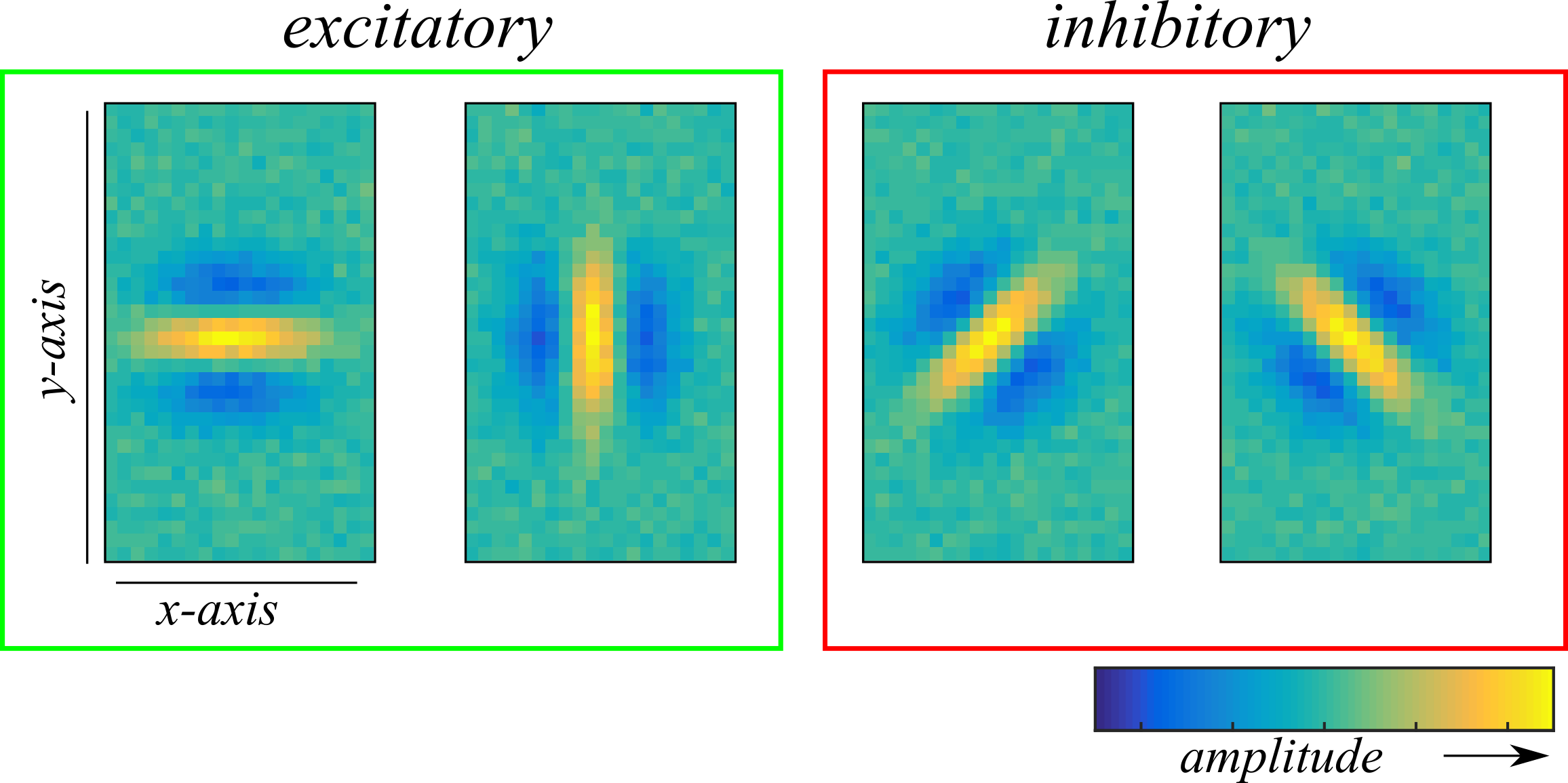
Consider an "edge-detecting" vision neuron whose responses signal the presence of vertical or horizontal edges in its field of view. The functional inputs of such a detector may look like those in Figure 1 where a vertical and horizontal gabor filter lead the neuron to elicit spikes while two diagonal Gabor filters inhibit the neurons response.

This neuron is subjected to white noise stimulation by a video of 200,000 frames presented at 60 Hz (the frame rate is arbitrary for this synthetic neuron). The thresholds for activation of the functional inputs are set such that the mean spike rate is \( \sim 0.25 \) spikes/frame.
As is usually done when identifying functional bases, the first step is to identify the receptive field of the neuron (the subspace of stimulus space relevant to the neural response). Since the neuron is subjected to white noise stimulation, a dimensionality reduction method known as spike-triggered covariance (STC) will suffice. STC is defined as follows:
where \(N_\mathrm{spk} = \sum_{t=1}^{N_\mathrm{samp}} y_t \) is the total response, \( N_\mathrm{samp} = 200000 \) is the total number of samples, \( \mathbf{s}_t \) is a stimulus sample vector (a frame from the video unrolled into a vector), \( y_t \) is the number of spikes or probability of a spike in response to stimulus sample \( t \), and \( \cdot^\mathrm{T} \) denotes a vector/matrix transpose. After constructing the matrix \( \mathbf{J} \), dimensionality reduction is achieved through the eigendecomposition of \( \mathbf{J} \) from which the four eigenvectors paired with the four largest magnitude eigenvalues recover a set of vectors that span the receptive field, \( \left\{ \boldsymbol{\omega}_k | \text{ for all } k \in \{ 1, \cdots, r \} \right\} \) where \( r = 4 \). The receptive field recovered via STC appears in Figure 2.
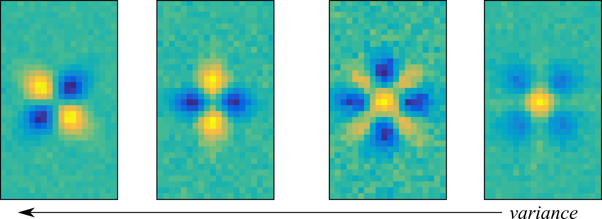
While the recovered receptive field approximately captures the same subspace of stimulus space as the ground truth in Figure 1, they cannot be taken at face value without giving us the wrong idea about the neural computation. In fact, it might be difficult to decide that linear combinations of these vectors must form a set of rotationally invariant Gabors, much less that two of the functional inputs are excitatory and the rest suppressive. We can, however, take advantage of dimensionality reduction by projecting the stimulus vectors into this subspace, \( s_{k,t} \leftarrow \boldsymbol{\omega}_{k} \cdot \mathbf{s}_t \) for all \( k \), to reduce the search space for nonconvex hypotheses of the functional basis.
Turning to the second step, the functional basis method, one might suspect correctly that logical OR and logical AND operations may not be the most appropriate when excitation and suppression is mixed. Logical OR has been found to correlate with purely excitatory inputs while logical AND correlates with completely suppressive inputs. Rather, it may be more appropriate to instead use a mixed logic gate of the form
which is a product of the \( P_\mathrm{OR} \) function from above with cardinality \( |C_\mathrm{OR}| = M \) and the \( P_\mathrm{AND} \) function with \( |C_\mathrm{AND}| = N \). The intuition here is that since either of the excitatory inputs can drive the neuron to spike, they may be best modeled by a logical OR function. However, since the suppressive dimensions can override the excitatory response and inhibit the neuron, a logical AND can sufficiently represent "off" inputs.
To test whether this hypothesis for the functional basis will best recover the functional basis, the data was split into 75% training and 25% cross-validation samples and mixed logic models enumerating all combinations of \( M \in \left\{ 1, \cdots, 4 \right\} \) and \( N \in \left\{ 1, \cdots, 4 \right\} \) were compared in their ability to predict responses on the cross-validation set. This procedure, called model selection, is presented in Figure 3 where the log-likelihood satures at the \( M = 2 \) and \( N = 2 \) model.
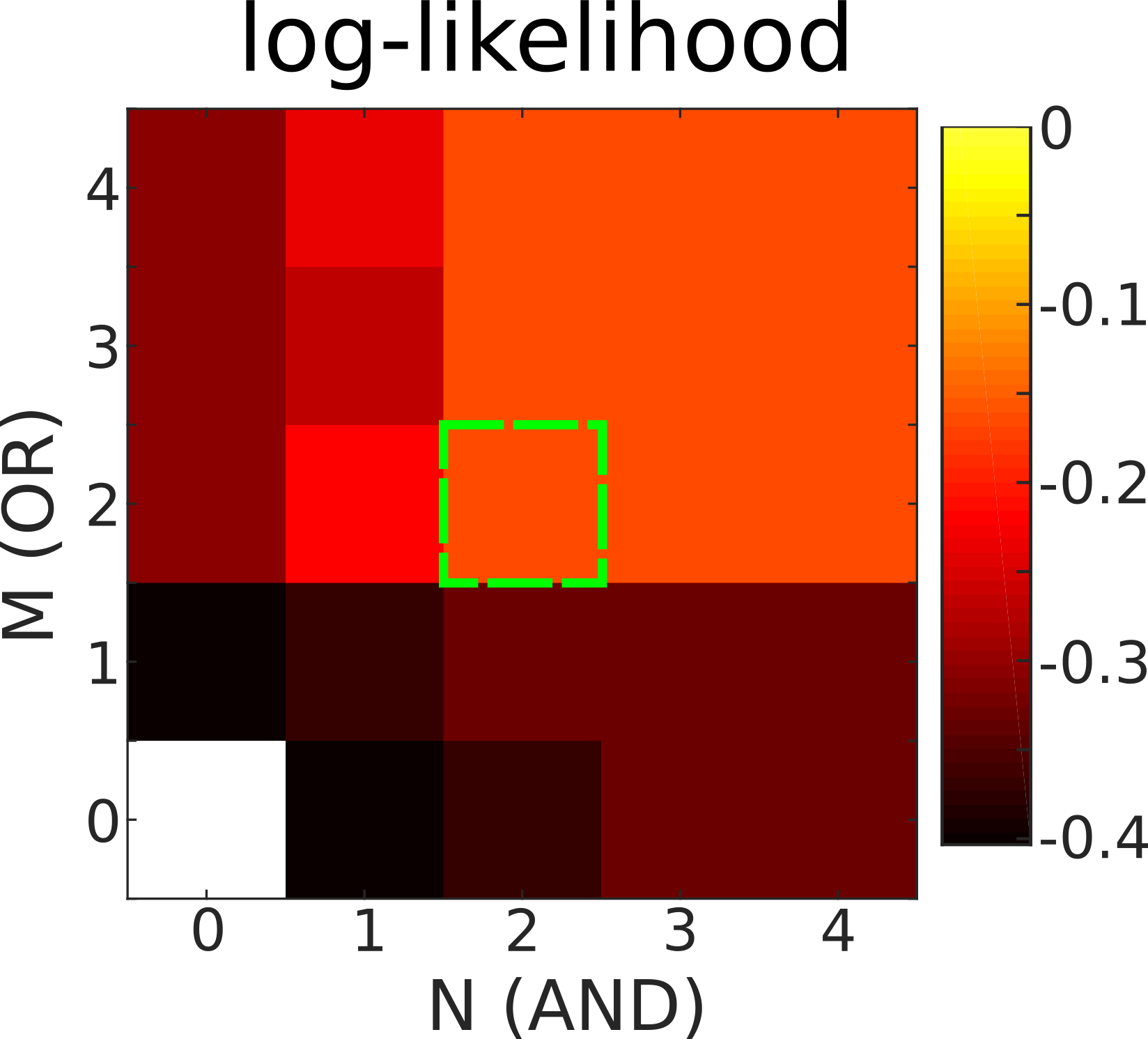
Since a larger log-likelihood indicates better predictions, this means that models where \( M \geq 2 \) and \( N \geq 2 \) all predict responses to the cross-validation set equally well. Of these, the best choice is the model that attains the best performance with the least number of parameters; i.e. the model that minimizes \( M + N \). Therefore, the best model is the \( M = 2 \) and \( N = 2\) model. Indeed, if we look at the functional inputs derived from the best model (expanded into the full stimulus space), we can see in Figure 4 that the recovered functional basis closely matches the ground truth functional inputs in Figure 1.
It can be concluded from this analysis that the proposed mixed Boolean operation is a satisfactory hypothesis for a neuron whose computation combines excitatory and suppressive inputs.